School Data, from Charnes et al. (1981), a large scale social experiment in public school education.
It was conceived in the late 1960's as a federally sponsored program charged with providing remedial
assistance to educationally disadvantaged early primary school students.
One aim is to explain scores on 3
different tests, reading, mathematics and selfesteem
from 70 school sites by means of 5 explanatory variables related to parents
and teachers.
Format
A data frame with 70 observations on the following 8 variables.
educationEducation level of mother as measured by the percentage of high school graduates among female parents
occupationHighest occupation of a family member according to a pre-arranged rating scale
visitParental visits index, representing the number of visits to the school site
counselingParent counseling index, calculated from data on time spent with child on school-related topics such as reading together, etc.
teacherNumber of teachers at the given site
readingReading score as measured by the Metropolitan Achievement Test
mathematicsMathematics score as measured by the Metropolitan Achievement Test
selfesteemCoopersmith Self-Esteem Inventory, intended as a measure of self-esteem
Details
A number of observations are unusual, a fact only revealed by plotting.
The study was designed to compare schools using Program Follow Through (PFT)
management methods of taking actions to achieve goals with those of
Non Follow Through (NFT). Observations 1:49 came from PFT sites
and 50:70 from NFT sites.
This and other descriptors are contained in the dataset schoolsites.
References
A. Charnes, W.W. Cooper and E. Rhodes (1981). Evaluating Program and Managerial Efficiency: An Application of Data Envelopment Analysis to Program Follow Through. Management Science, 27, 668-697.
Examples
data(schooldata)
# initial screening
plot(schooldata)
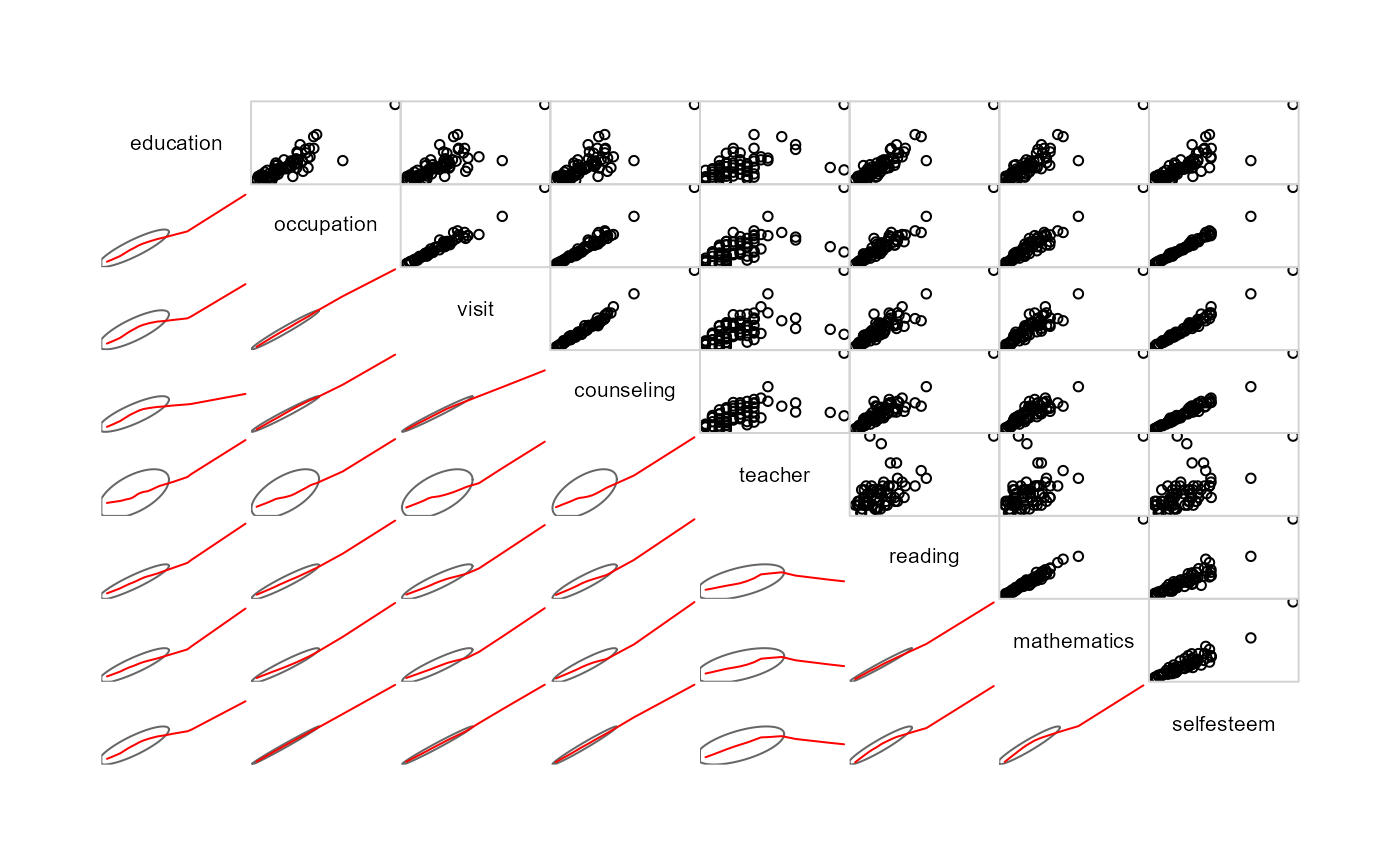
 # better plot
library(corrgram)
corrgram(schooldata,
lower.panel=panel.ellipse,
upper.panel=panel.pts)
# better plot
library(corrgram)
corrgram(schooldata,
lower.panel=panel.ellipse,
upper.panel=panel.pts)
 # check for multivariate outliers
res <- cqplot(schooldata, id.n = 5)
# check for multivariate outliers
res <- cqplot(schooldata, id.n = 5)
 res
#> DSQ quantile p
#> 59 44.58221 21.00172 0.007142857
#> 44 38.82543 17.97317 0.021428571
#> 33 27.92339 16.50356 0.035714286
#> 66 24.01111 15.50731 0.050000000
#> 35 21.73211 14.74557 0.064285714
#fit the MMreg model
school.mod <- lm(cbind(reading, mathematics, selfesteem) ~
education + occupation + visit + counseling + teacher, data=schooldata)
# shorthand: fit all others
school.mod <- lm(cbind(reading, mathematics, selfesteem) ~ ., data=schooldata)
car::Anova(school.mod)
#>
#> Type II MANOVA Tests: Pillai test statistic
#> Df test stat approx F num Df den Df Pr(>F)
#> education 1 0.37564 12.4337 3 62 1.820e-06 ***
#> occupation 1 0.56658 27.0159 3 62 2.687e-11 ***
#> visit 1 0.26032 7.2734 3 62 0.0002948 ***
#> counseling 1 0.06465 1.4286 3 62 0.2429676
#> teacher 1 0.04906 1.0661 3 62 0.3700291
#> ---
#> Signif. codes: 0 '***' 0.001 '**' 0.01 '*' 0.05 '.' 0.1 ' ' 1
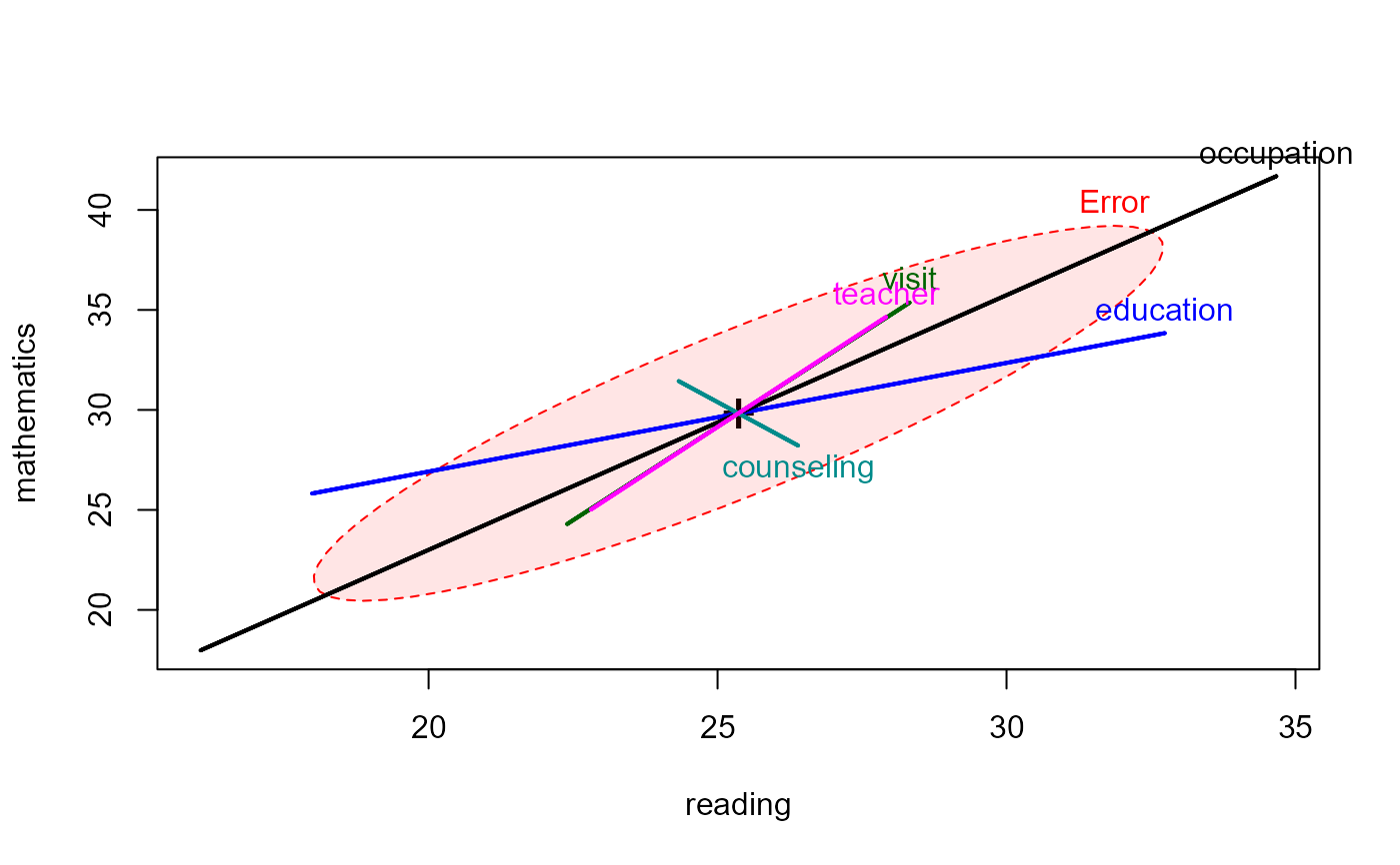
# HE plots
heplot(school.mod, fill=TRUE, fill.alpha=0.1)
res
#> DSQ quantile p
#> 59 44.58221 21.00172 0.007142857
#> 44 38.82543 17.97317 0.021428571
#> 33 27.92339 16.50356 0.035714286
#> 66 24.01111 15.50731 0.050000000
#> 35 21.73211 14.74557 0.064285714
#fit the MMreg model
school.mod <- lm(cbind(reading, mathematics, selfesteem) ~
education + occupation + visit + counseling + teacher, data=schooldata)
# shorthand: fit all others
school.mod <- lm(cbind(reading, mathematics, selfesteem) ~ ., data=schooldata)
car::Anova(school.mod)
#>
#> Type II MANOVA Tests: Pillai test statistic
#> Df test stat approx F num Df den Df Pr(>F)
#> education 1 0.37564 12.4337 3 62 1.820e-06 ***
#> occupation 1 0.56658 27.0159 3 62 2.687e-11 ***
#> visit 1 0.26032 7.2734 3 62 0.0002948 ***
#> counseling 1 0.06465 1.4286 3 62 0.2429676
#> teacher 1 0.04906 1.0661 3 62 0.3700291
#> ---
#> Signif. codes: 0 '***' 0.001 '**' 0.01 '*' 0.05 '.' 0.1 ' ' 1
# HE plots
heplot(school.mod, fill=TRUE, fill.alpha=0.1)
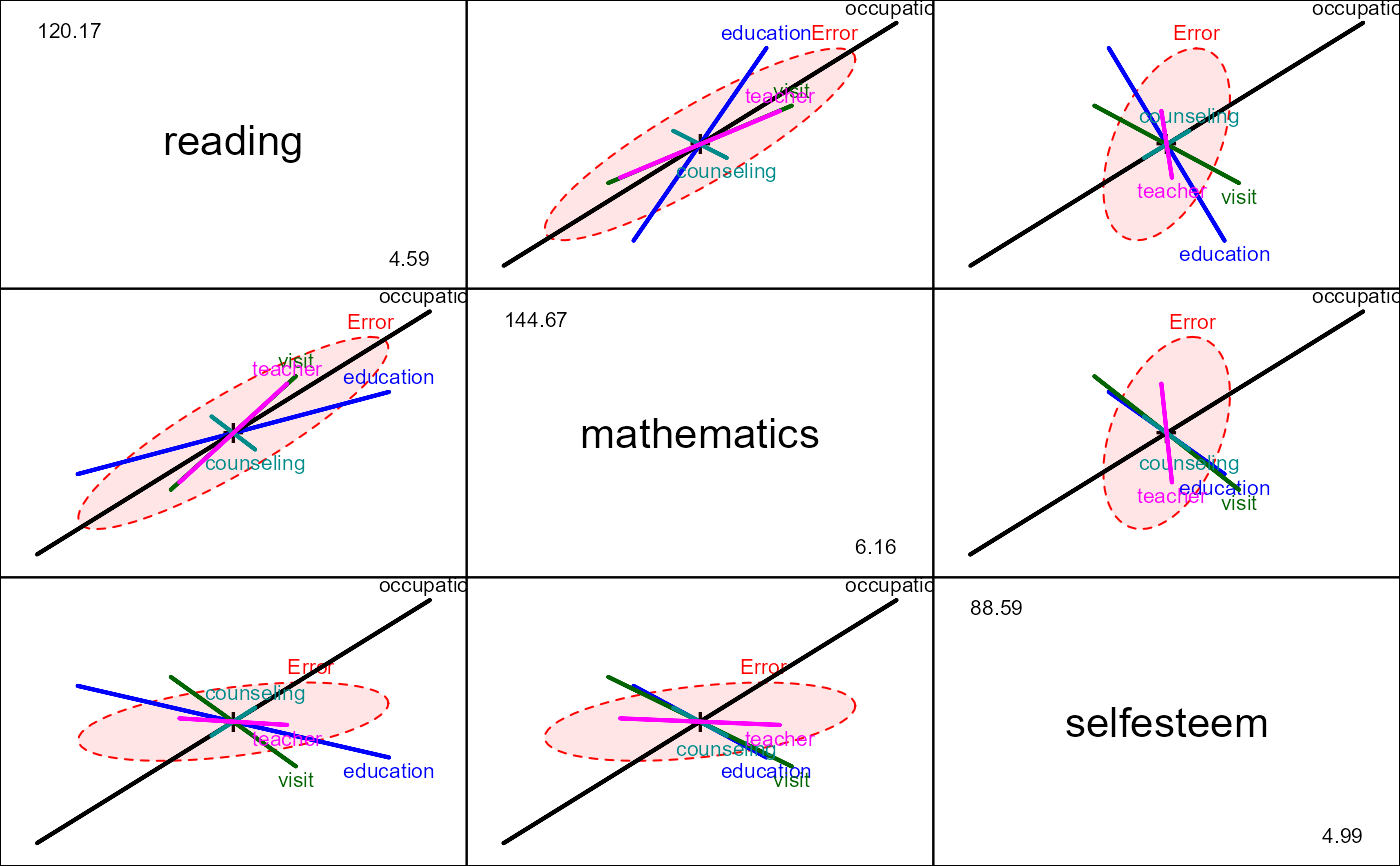 pairs(school.mod, fill=TRUE, fill.alpha=0.1)
 # robust model, using robmlm()
school.rmod <- robmlm(cbind(reading, mathematics, selfesteem) ~ ., data=schooldata)
# note that counseling is now significant
car::Anova(school.rmod)
#>
#> Type II MANOVA Tests: Pillai test statistic
#> Df test stat approx F num Df den Df Pr(>F)
#> education 1 0.39455 12.8161 3 59 1.488e-06 ***
#> occupation 1 0.59110 28.4301 3 59 1.683e-11 ***
#> visit 1 0.23043 5.8888 3 59 0.0013819 **
#> counseling 1 0.25257 6.6456 3 59 0.0006083 ***
#> teacher 1 0.09812 2.1395 3 59 0.1048263
#> ---
#> Signif. codes: 0 '***' 0.001 '**' 0.01 '*' 0.05 '.' 0.1 ' ' 1
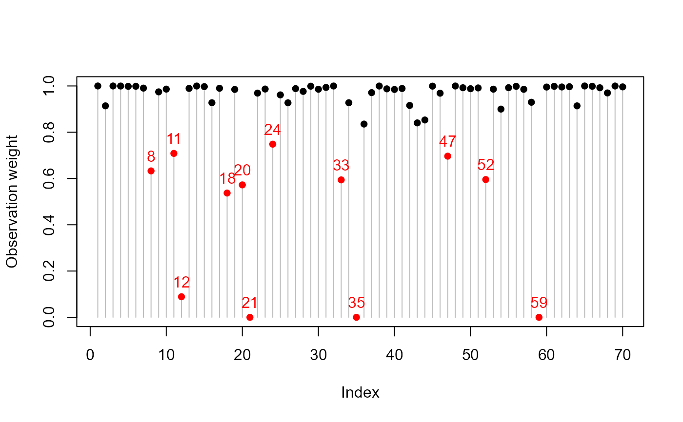
# Index plot of the weights
wts <- school.rmod$weights
notable <- which(wts < 0.8)
plot(wts, type = "h", col="gray", ylab = "Observation weight")
points(seq_along(wts), wts,
pch=16,
col = ifelse(wts < 0.8, "red", "black"))
text(notable, wts[notable],
labels = notable,
pos = 3,
col = "red")
# robust model, using robmlm()
school.rmod <- robmlm(cbind(reading, mathematics, selfesteem) ~ ., data=schooldata)
# note that counseling is now significant
car::Anova(school.rmod)
#>
#> Type II MANOVA Tests: Pillai test statistic
#> Df test stat approx F num Df den Df Pr(>F)
#> education 1 0.39455 12.8161 3 59 1.488e-06 ***
#> occupation 1 0.59110 28.4301 3 59 1.683e-11 ***
#> visit 1 0.23043 5.8888 3 59 0.0013819 **
#> counseling 1 0.25257 6.6456 3 59 0.0006083 ***
#> teacher 1 0.09812 2.1395 3 59 0.1048263
#> ---
#> Signif. codes: 0 '***' 0.001 '**' 0.01 '*' 0.05 '.' 0.1 ' ' 1
# Index plot of the weights
wts <- school.rmod$weights
notable <- which(wts < 0.8)
plot(wts, type = "h", col="gray", ylab = "Observation weight")
points(seq_along(wts), wts,
pch=16,
col = ifelse(wts < 0.8, "red", "black"))
text(notable, wts[notable],
labels = notable,
pos = 3,
col = "red")
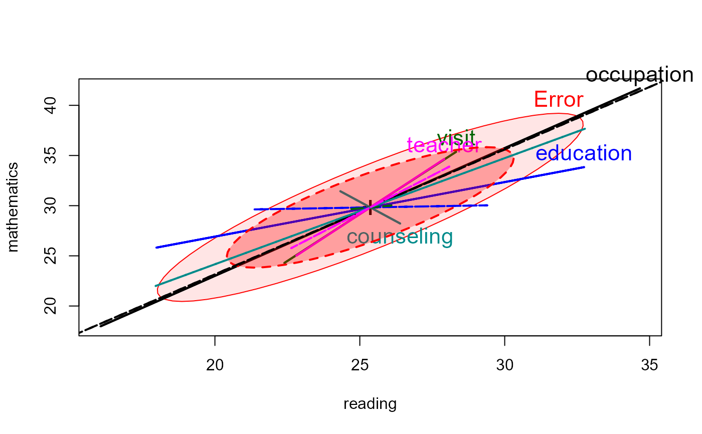
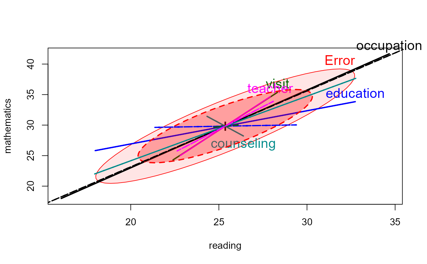 # compare classical HE plot with that based on the robust model
heplot(school.mod, cex=1.4, lty=1, fill=TRUE, fill.alpha=0.1)
heplot(school.rmod,
add=TRUE,
error.ellipse=TRUE,
lwd=c(2,2), lty=c(2,2),
term.labels=FALSE, err.label="",
fill=TRUE)
# compare classical HE plot with that based on the robust model
heplot(school.mod, cex=1.4, lty=1, fill=TRUE, fill.alpha=0.1)
heplot(school.rmod,
add=TRUE,
error.ellipse=TRUE,
lwd=c(2,2), lty=c(2,2),
term.labels=FALSE, err.label="",
fill=TRUE)