Plot method for regvec3d objects

The plot method for regvec3d objects uses the low-level graphics tools in this package to draw 3D and 3D vector diagrams reflecting the partial and marginal relations of y to x1 and x2 in a bivariate multiple linear regression model, lm(y ~ x1 + x2).

The summary method prints the vectors and their vector lengths, followed by the summary for the model.

Usage

# S3 method for class 'regvec3d'
plot(
  x,
  y,
  dimension = 3,
  col = c("black", "red", "blue", "brown", "lightgray"),
  col.plane = "gray",
  cex.lab = 1.2,
  show.base = 2,
  show.marginal = FALSE,
  show.hplane = TRUE,
  show.angles = TRUE,
  error.sphere = c("none", "e", "y.hat"),
  scale.error.sphere = x$scale,
  level.error.sphere = 0.95,
  grid = FALSE,
  add = FALSE,
  ...
)

# S3 method for class 'regvec3d'
summary(object, ...)

# S3 method for class 'regvec3d'
print(x, ...)

Arguments

x: A “regvec3d” object
y: Ignored; only included for compatibility with the S3 generic
dimension: Number of dimensions to plot: 3 (default) or 2
col: A vector of 5 colors. col[1] is used for the y and residual (e) vectors, and for x1 and x2; col[2] is used for the vectors y -> yhat and y -> e; col[3] is used for the vectors yhat -> b1 and yhat -> b2;
col.plane: Color of the base plane in a 3D plot or axes in a 2D plot
cex.lab: character expansion applied to vector labels. May be a number or numeric vector corresponding to the the rows of X, recycled as necessary.
show.base: If show.base > 0, draws the base plane in a 3D plot; if show.base > 1, the plane is drawn thicker
show.marginal: If TRUE also draws lines showing the marginal relations of y on x1 and on x2
show.hplane: If TRUE, draws the plane defined by y, yhat and the origin in the 3D
show.angles: If TRUE, draw and label the angle between the x1 and x2 and between y and yhat, corresponding respectively to the correlation between the xs and the multiple correlation
error.sphere: Plot a sphere (or in 2D, a circle) of radius proportional to the length of the residual vector, centered either at the origin ("e") or at the fitted-values vector ("y.hat"; the default is "none".)
scale.error.sphere: Whether to scale the error sphere if error.sphere="y.hat"; defaults to TRUE if the vectors representing the variables are scaled, in which case the oblique projections of the error spheres can represent confidence intervals for the coefficients; otherwise defaults to FALSE.
level.error.sphere: The confidence level for the error sphere, applied if scale.error.sphere=TRUE.
grid: If TRUE, draws a light grid on the base plane
add: If TRUE, add to the current plot; otherwise start a new rgl or plot window
...: Parameters passed down to functions [unused now]
object: A regvec3d object for the summary method

Value

None

Details

A 3D diagram shows the vector y and the plane formed by the predictors, x1 and x2, where all variables are represented in deviation form, so that the intercept need not be included.

A 2D diagram, using the first two columns of the result, can be used to show the projection of the space in the x1, x2 plane.

The drawing functions vectors and vectors3d used by the plot.regvec3d method only work reasonably well if the variables are shown on commensurate scales, i.e., with either scale=TRUE or normalize=TRUE.

References

Fox, J. (2016). Applied Regression Analysis and Generalized Linear Models, 3rd ed., Sage, Chapter 10.

Examples

if (require(carData)) {
   data("Duncan", package="carData")
   dunc.reg <- regvec3d(prestige ~ income + education, data=Duncan)
   plot(dunc.reg)
   plot(dunc.reg, dimension=2)
   plot(dunc.reg, error.sphere="e")
   summary(dunc.reg)

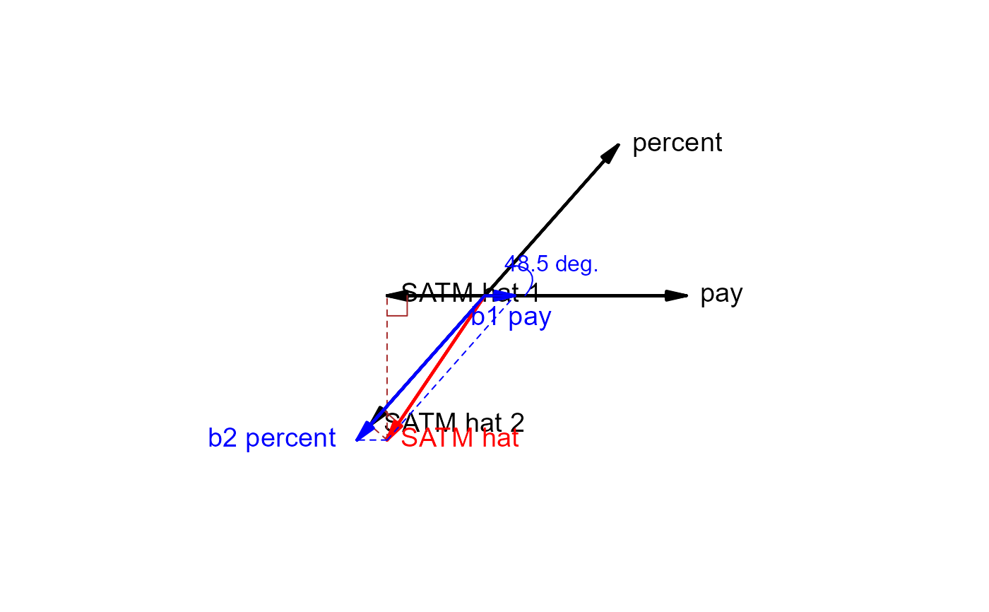
   # Example showing Simpson's paradox
   data("States", package="carData")
   states.vec <- regvec3d(SATM ~ pay + percent, data=States, scale=TRUE)
   plot(states.vec, show.marginal=TRUE)
   plot(states.vec, show.marginal=TRUE, dimension=2)
   summary(states.vec)
}
#> Loading required package: carData

#>                        x         y         z    length
#> income         0.7754622 0.0000000 0.0000000 0.7754622
#> education      0.6842863 0.6509930 0.0000000 0.9444785
#> prestige       0.8378014 0.3553340 0.4145197 1.0000000
#> residuals      0.0000000 0.0000000 0.4145197 0.4145197
#> prestige hat   0.8378014 0.3553340 0.0000000 0.9100403
#> b1 income      0.4642947 0.0000000 0.0000000 0.4642947
#> b2 education   0.3735067 0.3553340 0.0000000 0.5155284
#> prestige hat 1 0.8378014 0.0000000 0.0000000 0.8378014
#> prestige hat 2 0.6172234 0.5871929 0.0000000 0.8519156
#> 
#> Call:
#> lm(formula = formula, data = Data)
#> 
#> Residuals:
#>     Min      1Q  Median      3Q     Max 
#> -29.538  -6.417   0.655   6.605  34.641 
#> 
#> Coefficients:
#>             Estimate Std. Error t value Pr(>|t|)    
#> (Intercept) -6.06466    4.27194  -1.420    0.163    
#> income.      0.59873    0.11967   5.003 1.05e-05 ***
#> education.   0.54583    0.09825   5.555 1.73e-06 ***
#> ---
#> Signif. codes:  0 '***' 0.001 '**' 0.01 '*' 0.05 '.' 0.1 ' ' 1
#> 
#> Residual standard error: 13.37 on 42 degrees of freedom
#> Multiple R-squared:  0.8282,	Adjusted R-squared:   0.82 
#> F-statistic: 101.2 on 2 and 42 DF,  p-value: < 2.2e-16
#> 

#>                      x          y        z    length
#> pay          1.0000000  0.0000000 0.000000 1.0000000
#> percent      0.6630098  0.7486108 0.000000 1.0000000
#> SATM        -0.4853306 -0.7164880 0.501098 1.0000000
#> residuals    0.0000000  0.0000000 0.501098 0.5010980
#> SATM hat    -0.4853306 -0.7164880 0.000000 0.8653905
#> b1 pay       0.1492295  0.0000000 0.000000 0.1492295
#> b2 percent  -0.6345601 -0.7164880 0.000000 0.9570901
#> SATM hat 1  -0.4853306  0.0000000 0.000000 0.4853306
#> SATM hat 2  -0.5689615 -0.6424199 0.000000 0.8581495
#> 
#> Call:
#> lm(formula = formula, data = Data)
#> 
#> Residuals:
#>     Min      1Q  Median      3Q     Max 
#> -29.697 -13.788   0.701   9.988  42.961 
#> 
#> Coefficients:
#>             Estimate Std. Error t value Pr(>|t|)    
#> (Intercept) 513.6990    16.9174  30.365  < 2e-16 ***
#> pay.          0.9718     0.6292   1.545    0.129    
#> percent.     -1.3743     0.1387  -9.906 3.45e-13 ***
#> ---
#> Signif. codes:  0 '***' 0.001 '**' 0.01 '*' 0.05 '.' 0.1 ' ' 1
#> 
#> Residual standard error: 17.68 on 48 degrees of freedom
#> Multiple R-squared:  0.7489,	Adjusted R-squared:  0.7384 
#> F-statistic: 71.58 on 2 and 48 DF,  p-value: 3.947e-15
#>