Variance Inflation Factors for Ridge Regression

The function vif.ridge calculates variance inflation factors for the predictors in a set of ridge regression models indexed by the tuning/shrinkage factor.

Usage

# S3 method for ridge
vif(mod, ...)

Arguments

mod: A ridge object
...: Other arguments (unused)

Value

Returns a matrix of variance inflation factors of the same size and shape as coef{mod}. The columns correspond to the predictors in the model and the rows correspond to the values of lambda in ridge estimation.

Details

Variance inflation factors are calculated using the simplified formulation in Fox & Monette (1992).

References

Fox, J. and Monette, G. (1992). Generalized collinearity diagnostics. JASA, 87, 178-183

Author

Michael Friendly

Examples


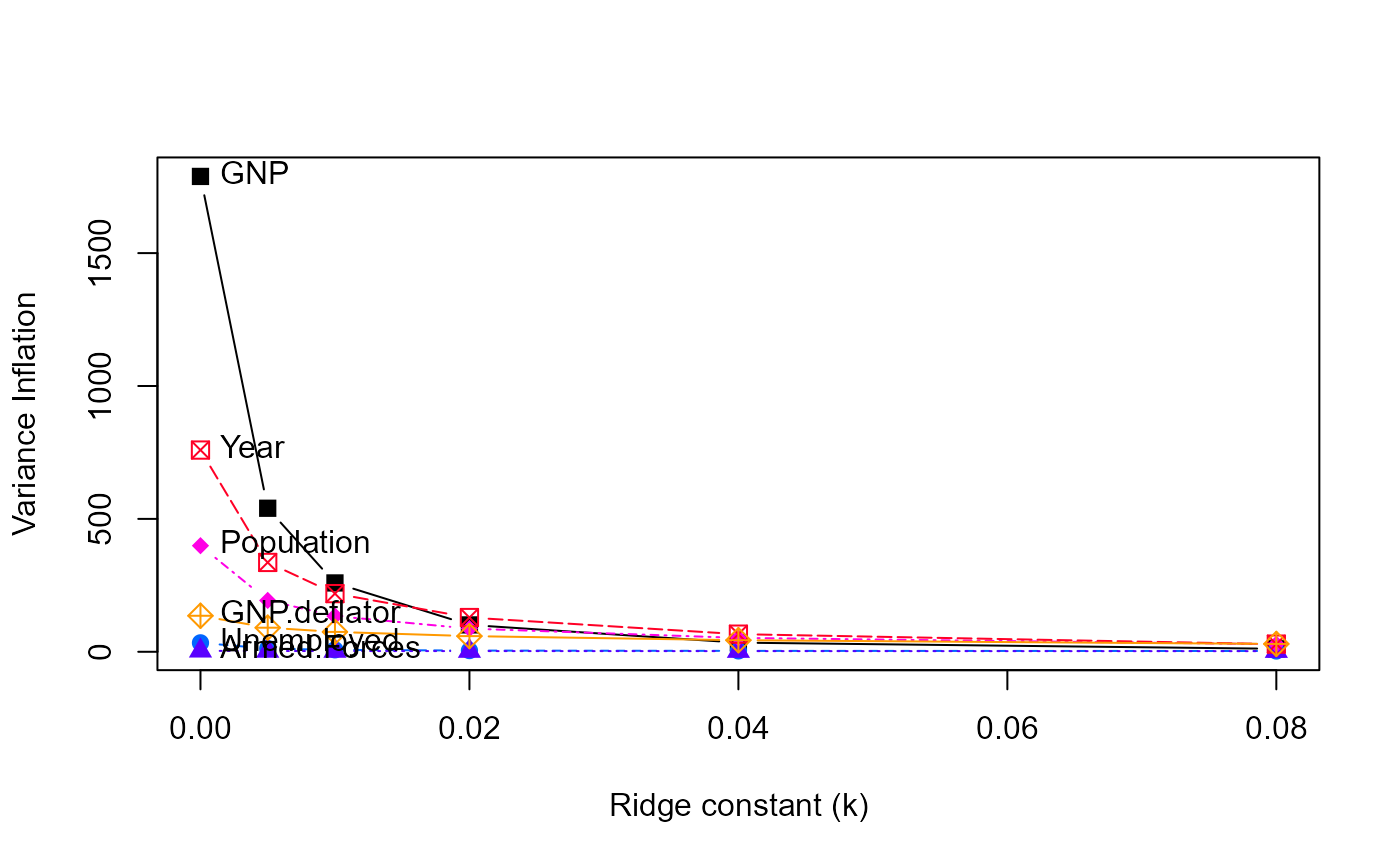
data(longley)
lmod <- lm(Employed ~ GNP + Unemployed + Armed.Forces + Population + 
                      Year + GNP.deflator, data=longley)
vif(lmod)
#>          GNP   Unemployed Armed.Forces   Population         Year GNP.deflator 
#>   1788.51348     33.61889      3.58893    399.15102    758.98060    135.53244 

longley.y <- longley[, "Employed"]
longley.X <- data.matrix(longley[, c(2:6,1)])

lambda <- c(0, 0.005, 0.01, 0.02, 0.04, 0.08)
lridge <- ridge(longley.y, longley.X, lambda=lambda)
coef(lridge)
#>              GNP Unemployed Armed.Forces  Population     Year GNP.deflator
#> 0.000 -3.4471925  -1.827886   -0.6962102 -0.34419721 8.431972   0.15737965
#> 0.005 -1.0424783  -1.491395   -0.6234680 -0.93558040 6.566532  -0.04175039
#> 0.010 -0.1797967  -1.361047   -0.5881396 -1.00316772 5.656287  -0.02612152
#> 0.020  0.4994945  -1.245137   -0.5476331 -0.86755299 4.626116   0.09766305
#> 0.040  0.9059471  -1.155229   -0.5039108 -0.52347060 3.576502   0.32123994
#> 0.080  1.0907048  -1.086421   -0.4582525 -0.08596324 2.641649   0.57025165


vridge <- vif(lridge)
vridge
#>              GNP Unemployed Armed.Forces Population      Year GNP.deflator
#> 0.000 1788.51348  33.618891     3.588930  399.15102 758.98060    135.53244
#> 0.005  540.04391  12.118058     2.920757  193.29890 336.15377     90.62954
#> 0.010  258.99935   7.284398     2.732975  134.42069 218.84254     74.78548
#> 0.020  101.11696   4.572957     2.577977   87.29189 128.82070     58.93518
#> 0.040   34.42567   3.422139     2.440659   52.22396  66.31015     43.55638
#> 0.080   11.28144   2.994018     2.301110   28.59266  28.82089     29.52231

# plot VIFs
pch <- c(15:18, 7, 9)
clr <- c("black", rainbow(5, start=.6, end=.1))

matplot(rownames(vridge), vridge, type='b', 
  xlab='Ridge constant (k)', ylab="Variance Inflation", 
  xlim=c(0, 0.08), 
  col=clr, pch=pch, cex=1.2)
text(0.0, vridge[1,], colnames(vridge), pos=4)


matplot(lridge$df, vridge, type='b', 
  xlab='Degrees of freedom', ylab="Variance Inflation", 
  col=clr, pch=pch, cex=1.2)
text(6, vridge[1,], colnames(vridge), pos=2)


# more useful to plot VIF on the sqrt scale

matplot(rownames(vridge), sqrt(vridge), type='b', 
  xlab='Ridge constant (k)', ylab=expression(sqrt(VIF)), 
  xlim=c(-0.01, 0.08), 
  col=clr, pch=pch, cex=1.2, cex.lab=1.25)
text(-0.01, sqrt(vridge[1,]), colnames(vridge), pos=4, cex=1.2)


matplot(lridge$df, sqrt(vridge), type='b', 
  xlab='Degrees of freedom', ylab=expression(sqrt(VIF)), 
  col=clr, pch=pch, cex=1.2, cex.lab=1.25)
text(6, sqrt(vridge[1,]), colnames(vridge), pos=2, cex=1.2)