Influence Index Plots for Multivariate Linear Models

Provides index plots of some diagnostic measures for a multivariate linear model: Cook's distance, a generalized (squared) studentized residual, hat-values (leverages), and Mahalanobis squared distances of the residuals.

Usage

# S3 method for mlm
infIndexPlot(
  model,
  infl = mlm.influence(model, do.coef = FALSE),
  FUN = det,
  vars = c("Cook", "Studentized", "hat", "DSQ"),
  main = paste("Diagnostic Plots for", deparse(substitute(model))),
  pch = 19,
  labels,
  id.method = "y",
  id.n = if (id.method[1] == "identify") Inf else 0,
  id.cex = 1,
  id.col = palette()[1],
  id.location = "lr",
  grid = TRUE,
  ...
)

Arguments

model: A multivariate linear model object of class mlm .
infl: influence measure structure as returned by mlm.influence
FUN: For m>1, the function to be applied to the \(H\) and \(Q\) matrices returning a scalar value. FUN=det and FUN=tr are possible choices, returning the \(|H|\) and \(tr(H)\) respectively.
vars: All the quantities listed in this argument are plotted. Use "Cook" for generalized Cook's distances, "Studentized" for generalized Studentized residuals, "hat" for hat-values (or leverages), and DSQ for the squared Mahalanobis distances of the model residuals. Capitalization is optional. All may be abbreviated by the first one or more letters.
main: main title for graph
pch: Plotting character for points
id.method, labels, id.n, id.cex, id.col, id.location: Arguments for the labeling of points. The default is id.n=0 for labeling no points. See showLabels for details of these arguments.
grid: If TRUE, the default, a light-gray background grid is put on the graph
...: Arguments passed to plot

Value

None. Used for its side effect of producing a graph.

Details

This function produces index plots of the various influence measures calculated by influence.mlm, and in addition, the measure based on the Mahalanobis squared distances of the residuals from the origin.

References

Barrett, B. E. and Ling, R. F. (1992). General Classes of Influence Measures for Multivariate Regression. Journal of the American Statistical Association, 87(417), 184-191.

Barrett, B. E. (2003). Understanding Influence in Multivariate Regression Communications in Statistics - Theory and Methods, 32, 667-680.

Author

Michael Friendly; borrows code from car::infIndexPlot

Examples


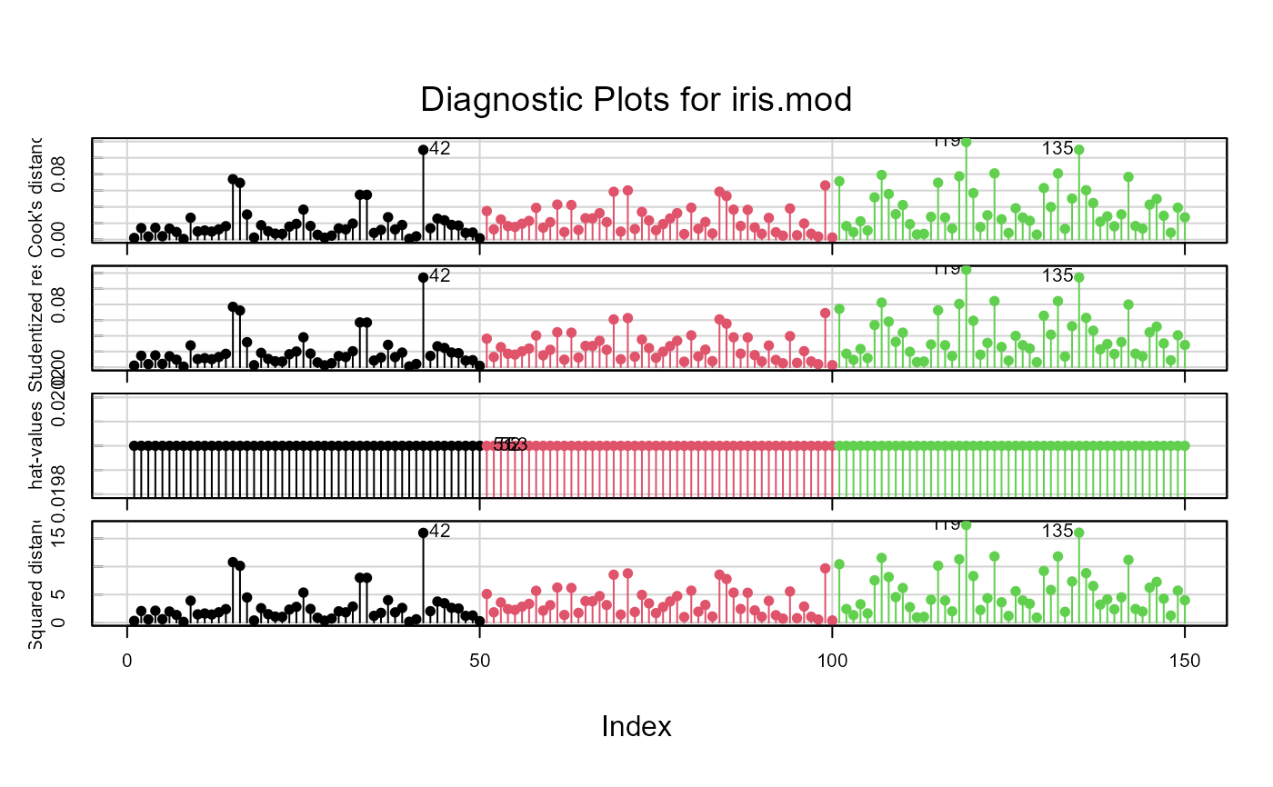
# iris data
data(iris)
iris.mod <- lm(as.matrix(iris[,1:4]) ~ Species, data=iris)
infIndexPlot(iris.mod, col=iris$Species, id.n=3)


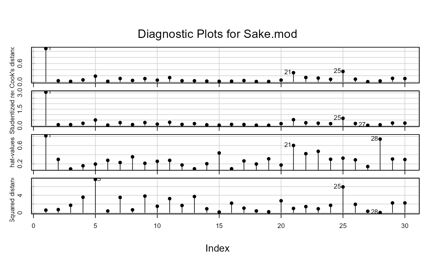
# Sake data
data(Sake, package="heplots")
Sake.mod <- lm(cbind(taste,smell) ~ ., data=Sake)
infIndexPlot(Sake.mod, id.n=3)


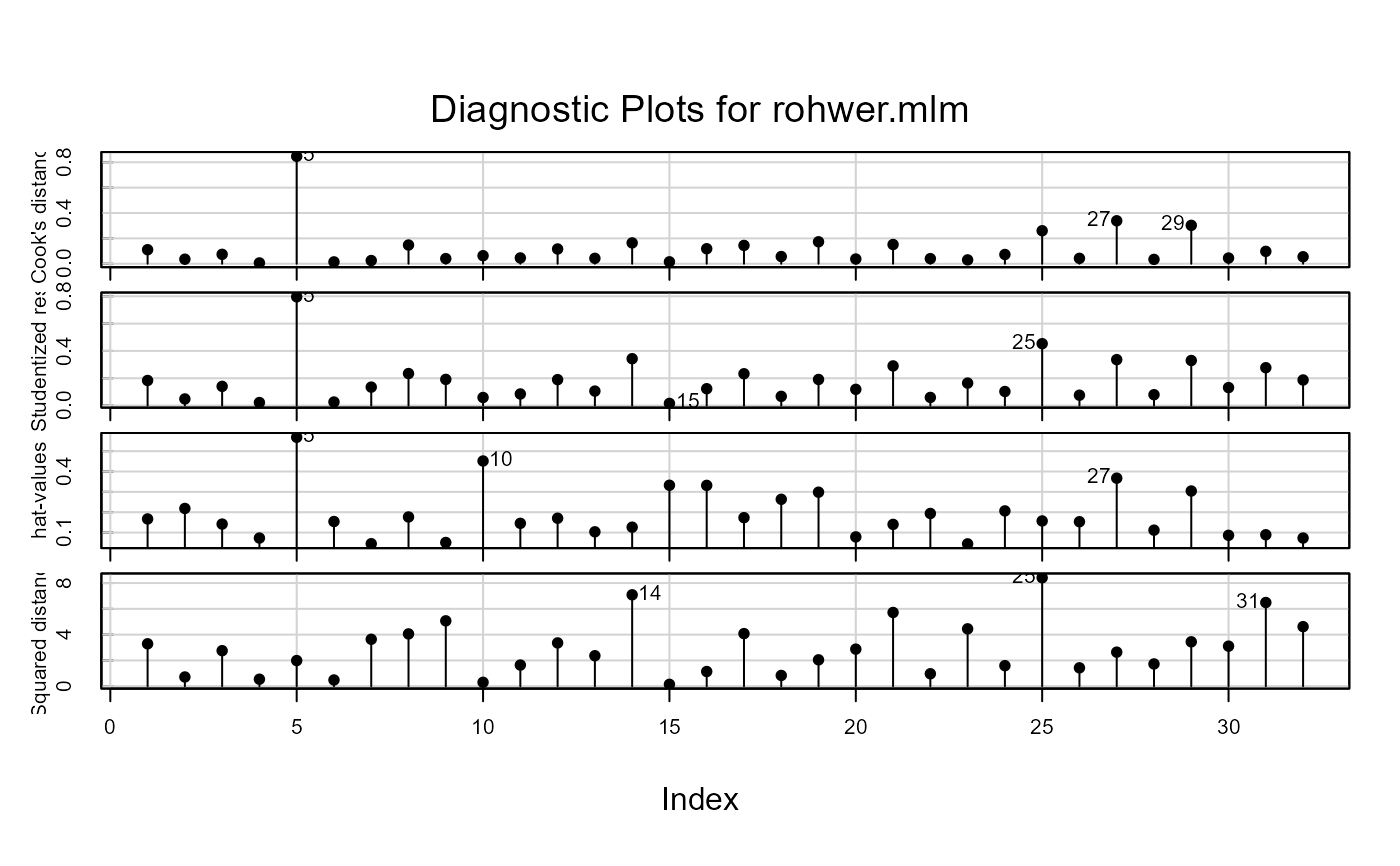
# Rohwer data
data(Rohwer, package="heplots")
Rohwer2 <- subset(Rohwer, subset=group==2)
rownames(Rohwer2)<- 1:nrow(Rohwer2)
rohwer.mlm <- lm(cbind(SAT, PPVT, Raven) ~ n + s + ns + na + ss, data=Rohwer2)
infIndexPlot(rohwer.mlm, id.n=3)