Using easystats with nestedLogit models

Michael Friendly

2026-03-04

Overview

The easystats project (easystats2022?) is a collection of R packages that provides a unified, consistent framework for working with statistical models. Three of its core packages offer direct support for "nestedLogit" objects:

• insight (R-insight?): Extracts model information — formulas, data, parameters, variance-covariance matrices — through a unified interface.
• parameters (R-parameters?): Computes and formats model parameter tables with confidence intervals, standardized coefficients, and bootstrap estimates.
• performance (R-performance?): Calculates model performance indices such as R-squared measures and fit statistics.

These packages work by iterating over the individual binary logit sub-models that comprise a nested dichotomy model, combining the results into tidy tables with a Response column identifying each dichotomy. This means you get a unified view of all dichotomies without having to process them individually.

Additionally, the see package provides plot() methods for the output of parameters and performance, enabling visual summaries like forest plots.

This vignette describes some ways to enhance what is available in the nestedLogit package using easystats capabilities.

Load the packages we’ll use here:

library(nestedLogit)    # Nested Dichotomy Logistic Regression Models
library(insight)        # Easy Access to Model Information
library(parameters)     # Processing of Model Parameters
library(performance)    # Assessment of Regression Models Performance
library(see)            # Visualisation Toolbox for easystats
library(ggplot2)        # Data Visualisations Using the Grammar of Graphics

Women’s labor force participation

We use the standard Womenlf example. The response partic has three categories — not working, working part-time, and working full-time — modeled as nested dichotomies against husband’s income and presence of young children.

data(Womenlf, package = "carData")
comparisons <- logits(work = dichotomy("not.work", c("parttime", "fulltime")),
                      full = dichotomy("parttime", "fulltime"))

wlf.nested <- nestedLogit(partic ~ hincome + children,
                          dichotomies = comparisons,
                          data = Womenlf)

Model information with insight

The insight package provides accessor functions that work uniformly across many model types. For nestedLogit models, these extract information from the overall model and, where applicable, from each dichotomy sub-model.

Model type and formula

model_info() retrieves information about a given model. The model family (binomial) and link function (logit) are recorded, as well as various is_* properties.

info <- insight::model_info(wlf.nested)

names(info)
#>  [1] "is_binomial"      "is_bernoulli"     "is_count"         "is_poisson"      
#>  [5] "is_negbin"        "is_beta"          "is_betabinomial"  "is_orderedbeta"  
#>  [9] "is_dirichlet"     "is_exponential"   "is_logit"         "is_probit"       
#> [13] "is_censored"      "is_truncated"     "is_survival"      "is_linear"       
#> [17] "is_tweedie"       "is_zeroinf"       "is_zero_inflated" "is_dispersion"   
#> [21] "is_hurdle"        "is_ordinal"       "is_cumulative"    "is_multinomial"  
#> [25] "is_categorical"   "is_mixed"         "is_multivariate"  "is_trial"        
#> [29] "is_bayesian"      "is_gam"           "is_anova"         "is_timeseries"   
#> [33] "is_ttest"         "is_correlation"   "is_onewaytest"    "is_chi2test"     
#> [37] "is_ranktest"      "is_levenetest"    "is_variancetest"  "is_xtab"         
#> [41] "is_proptest"      "is_binomtest"     "is_ftest"         "is_meta"         
#> [45] "is_wiener"        "is_rtchoice"      "is_mixture"       "link_function"   
#> [49] "family"           "n_obs"            "n_grouplevels"

The relevant values here are:

info$is_binomial
#> [1] TRUE
info$family
#> [1] "binomial"
info$link_function
#> [1] "logit"

find_formula() returns the model formula. With dichotomies = TRUE, it returns the formula for each sub-model:

insight::find_formula(wlf.nested)
#> $conditional
#> partic ~ hincome + children
#> 
#> attr(,"class")
#> [1] "insight_formula" "list"
insight::find_formula(wlf.nested, dichotomies = TRUE)
#> $work
#> $conditional
#> work ~ hincome + children
#> 
#> attr(,"class")
#> [1] "insight_formula" "list"           
#> 
#> $full
#> $conditional
#> full ~ hincome + children
#> 
#> attr(,"class")
#> [1] "insight_formula" "list"

Parameters and data

find_parameters() lists all parameter names across the dichotomies:

insight::find_parameters(wlf.nested)
#> $conditional
#> [1] "(Intercept)"     "hincome"         "childrenpresent"

get_varcov() returns the variance-covariance matrix for each sub-model. The component argument lets you select a specific dichotomy:

insight::get_varcov(wlf.nested)
#> $work
#>                 (Intercept)    hincome childrenpresent
#> (Intercept)        0.147274 -0.0058877      -0.0645454
#> hincome           -0.005888  0.0003913       0.0003901
#> childrenpresent   -0.064545  0.0003901       0.0854176
#> 
#> $full
#>                 (Intercept)   hincome childrenpresent
#> (Intercept)         0.58846 -0.025136       -0.286297
#> hincome            -0.02514  0.001533        0.006708
#> childrenpresent    -0.28630  0.006708        0.292762

Model parameters with parameters

Basic parameter table

The model_parameters() function produces a formatted summary of all coefficients across the dichotomies. The printed output includes estimates, standard errors, confidence intervals, and test statistics. The data structure contains a Response column identifying which dichotomy each row belongs to:

mp <- model_parameters(wlf.nested)
mp
#> # {not.work} vs. {parttime, fulltime} response
#> 
#> Parameter          | Log-Odds |   SE |         95% CI |     z |      p
#> ----------------------------------------------------------------------
#> (Intercept)        |     1.34 | 0.38 | [ 0.61,  2.12] |  3.48 | < .001
#> hincome            |    -0.04 | 0.02 | [-0.08,  0.00] | -2.14 | 0.032 
#> children [present] |    -1.58 | 0.29 | [-2.16, -1.01] | -5.39 | < .001
#> 
#> # {parttime} vs. {fulltime} response
#> 
#> Parameter          | Log-Odds |   SE |         95% CI |     z |      p
#> ----------------------------------------------------------------------
#> (Intercept)        |     3.48 | 0.77 | [ 2.11,  5.14] |  4.53 | < .001
#> hincome            |    -0.11 | 0.04 | [-0.19, -0.04] | -2.74 | 0.006 
#> children [present] |    -2.65 | 0.54 | [-3.80, -1.66] | -4.90 | < .001

Plot of coefficients

The see package provides a plot() method for parameter tables, producing a forest plot of the coefficient estimates with confidence intervals. This is intended to give a visual comparison of the effects across the two dichotomies.

There is a small incompatibility to work around:

• see::plot.parameters_model() internally passes Response column values to gsub() as regular expression patterns.
• The curly-brace notation that nestedLogit uses to label multi-category dichotomy sides (e.g., {parttime} vs. {fulltime}) contains { and } characters that are invalid regex quantifiers, causing an error.
• Stripping the braces before plotting resolves this:

mp_plot <- mp
mp_plot$Response <- gsub("[{}]", "", mp_plot$Response)
plot(mp_plot)

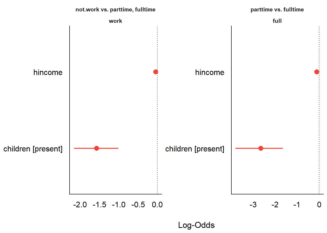
Forest plot of model coefficients from model_parameters().

Note that the two predictors are on very different scales: hincome is a continuous variable (measured in thousands of dollars) while children is binary (present/absent). This makes direct visual comparison of their coefficient sizes within the same panel potentially misleading. The model_parameters() function offers a standardize = "refit" argument that re-fits the model on z-scored predictors, which would put all coefficients on a common standard-deviation scale.

Unfortunately, this option does not currently produce a visibly different result for nestedLogit objects, suggesting that standardization is not yet fully propagated through the nested structure. Until this is resolved, the compare_parameters() approach in the next section — which works directly on the individual glm sub-models — is more reliable for visual comparison.

Comparing dichotomies

compare_parameters() places the estimates from different sub-models side by side, making it easy to see how the same predictors operate differently across the nested dichotomies. Here we extract the individual glm sub-models using models() and compare them:

cp <- compare_parameters(models(wlf.nested, "work"),
                         models(wlf.nested, "full"),
                         column_names = c("Work", "Full"))
cp
#> Parameter          |                 Work |                 Full
#> ----------------------------------------------------------------
#> (Intercept)        |  1.34 ( 0.58,  2.09) |  3.48 ( 1.97,  4.98)
#> hincome            | -0.04 (-0.08,  0.00) | -0.11 (-0.18, -0.03)
#> children [present] | -1.58 (-2.15, -1.00) | -2.65 (-3.71, -1.59)
#> ----------------------------------------------------------------
#> Observations       |                  263 |                  108

There is a plot method for the result, which plots the coefficients for the two sup-models in a single plot.

plot(cp)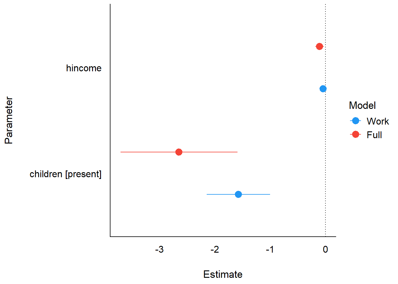

Comparison of coefficients across the two dichotomy sub-models.

Bootstrap confidence intervals

model_parameters() supports bootstrap-based inference. This re-fits the model on resampled data to produce non-parametric bootstrap confidence intervals, which can be more robust than the default Wald intervals for smaller samples:

model_parameters(wlf.nested, bootstrap = TRUE, iterations = 500)
#> # Fixed Effects
#> 
#> Parameter            | Log-Odds |         95% CI |      p
#> ---------------------------------------------------------
#> (Intercept).work     |     1.34 | [ 0.61,  2.18] | < .001
#> hincome.work         |    -0.04 | [-0.09,  0.00] | 0.044 
#> childrenpresent.work |    -1.60 | [-2.24, -1.08] | < .001
#> (Intercept).full     |     3.55 | [ 2.34,  5.43] | < .001
#> hincome.full         |    -0.11 | [-0.19, -0.05] | < .001
#> childrenpresent.full |    -2.72 | [-4.23, -1.75] | < .001

Model performance with performance

Performance summary

model_performance() provides a one-line summary of fit statistics for each dichotomy sub-model, including AIC, BIC, Tjur’s R-squared, RMSE, and log-likelihood:

model_performance(wlf.nested)
#> # Indices of model performance
#> 
#> Response |   AIC |   BIC |  RMSE | Sigma |    R2
#> ------------------------------------------------
#> work     | 325.7 | 336.4 | 0.456 |     1 | 0.138
#> full     | 110.5 | 118.5 | 0.398 |     1 | 0.333

R-squared measures

Several R-squared variants are available for logistic regression models. Tjur’s R-squared (also known as the coefficient of discrimination) is the default for binomial models:

r2(wlf.nested)
#> # R2 for Logistic Regression
#>   work: 0.138
#>    full: 0.333

Other R-squared measures provide alternative perspectives on model fit:

r2_nagelkerke(wlf.nested)
#> $work
#> Nagelkerke's R2 
#>          0.1743 
#> 
#> $full
#> Nagelkerke's R2 
#>          0.4185
r2_coxsnell(wlf.nested)
#> $work
#> Cox & Snell's R2 
#>           0.1293 
#> 
#> $full
#> Cox & Snell's R2 
#>           0.3085

Diagnostics for individual dichotomies

While the easystats functions above work on the nestedLogit object as a whole, some diagnostic tools (such as check_model()) require a standard glm object. The models() function extracts individual dichotomy sub-models, which are ordinary glm objects that work with the full range of easystats diagnostic tools.

Extracting sub-models

wlf_work <- models(wlf.nested, "work")  # working vs. not working
wlf_full <- models(wlf.nested, "full")  # full-time vs. part-time

class(wlf_work)
#> [1] "glm" "lm"

Visual diagnostics with check_model()

performance::check_model() produces a comprehensive set of diagnostic plots for a glm object, including checks for influential observations, collinearity, and the distribution of residuals.

check_model(wlf_work)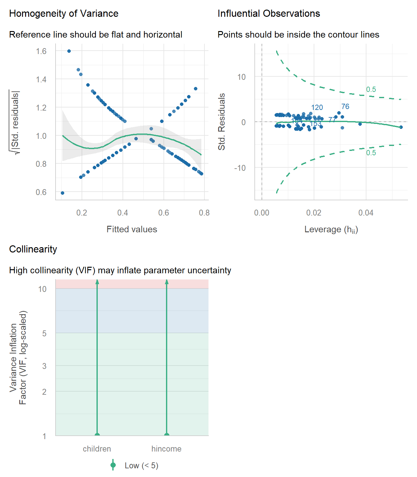

Diagnostic plots for the work vs. not-work dichotomy.

check_model(wlf_full)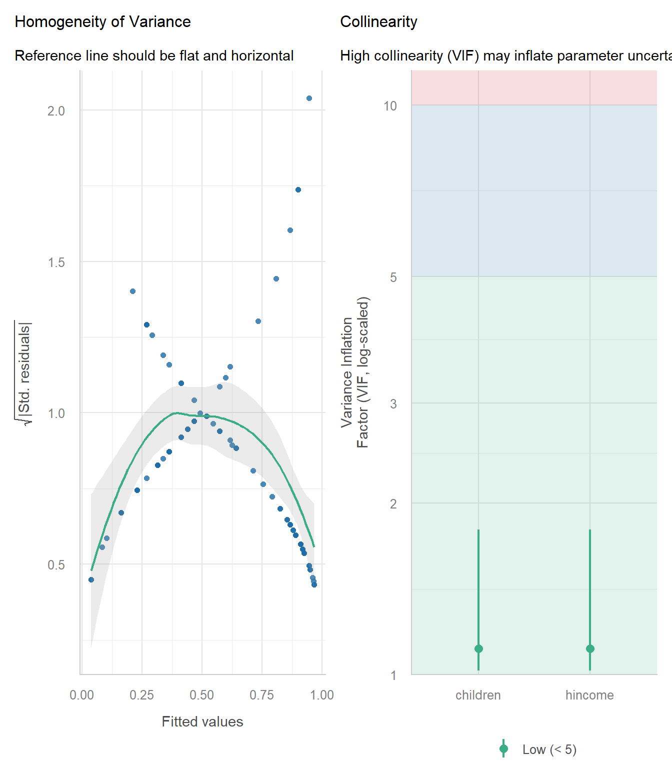

Diagnostic plots for the full-time vs. part-time dichotomy.

Binned residual plot

For binomial models, performance::binned_residuals() provides a binned residual plot, a more appropriate residual diagnostic than raw residuals. Points falling outside the error bounds suggest potential model misfit.

binned_residuals() requires the binary response variable to be present as a named column in the model’s data. The sub-models returned by models() have their call$data reset to the original dataset (Womenlf), which does not contain the binary response columns — those were created internally as a temporary variable during model fitting and were never added back to the original data. As a result, insight::get_data() cannot find the response column and errors.

The workaround is to construct small data frames with the binary response defined explicitly, matching the logic used by nestedLogit internally:

# work dichotomy: all cases, not.work = 0, parttime or fulltime = 1
df_work <- within(Womenlf, work <- as.integer(partic != "not.work"))
glm_work2 <- glm(work ~ hincome + children, data = df_work, family = binomial)
check_work <- binned_residuals(glm_work2)
plot(check_work)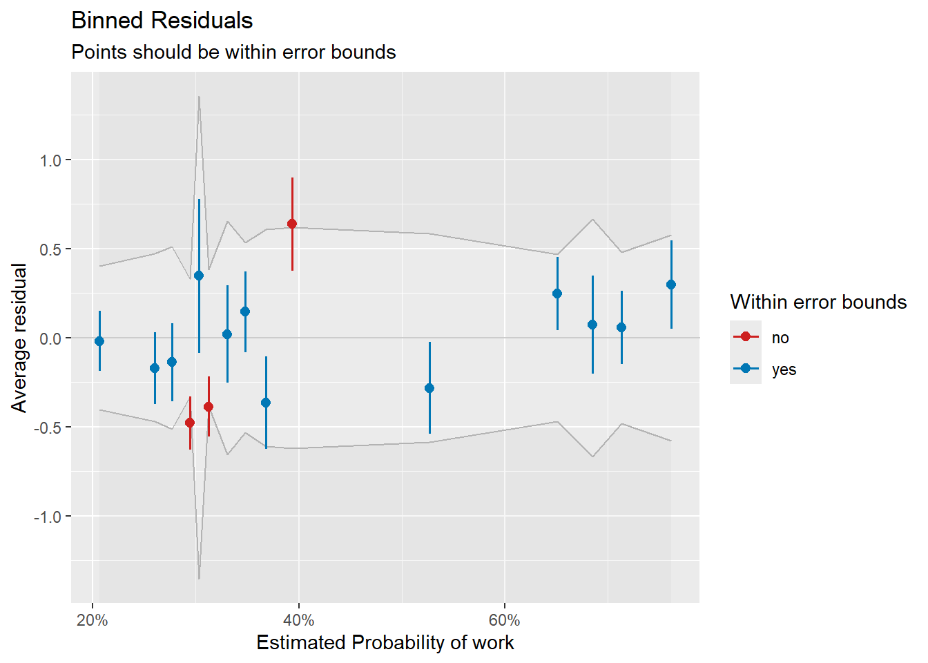

Binned residual plot for the work vs. not-work dichotomy.

# full dichotomy: workers only, parttime = 0, fulltime = 1
df_full <- subset(Womenlf, partic != "not.work")
df_full$full <- as.integer(df_full$partic == "fulltime")
glm_full2 <- glm(full ~ hincome + children, data = df_full, family = binomial)
check_full <- binned_residuals(glm_full2)
plot(check_full)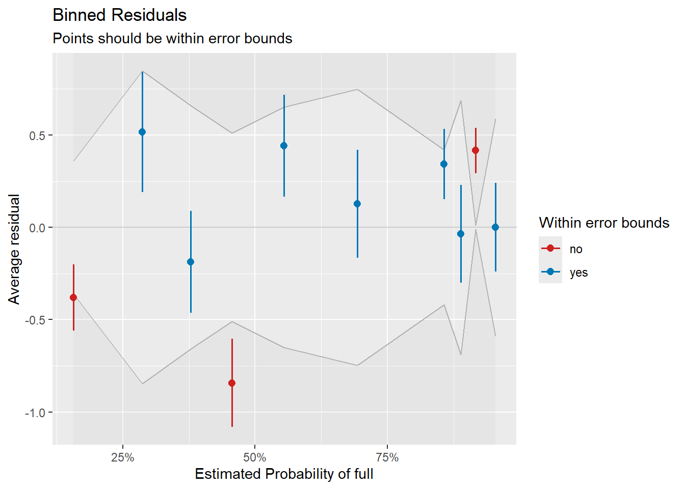

Binned residual plot for the full-time vs. part-time dichotomy.

Limitations

The easystats ecosystem provides substantial support for nestedLogit models through insight, parameters, and performance. However, some packages in the ecosystem do not currently support nestedLogit:

• modelbased: Functions like estimate_expectation() and estimate_prediction() do not work with nestedLogit objects. For predicted probabilities and marginal effects, use the ggeffects package instead (see vignette("ggeffects", package = "nestedLogit")).

• Diagnostic plots: check_model() does not work directly on nestedLogit objects, but as shown above, it can be applied to the individual glm sub-models extracted with models().

For plotting predicted probabilities of the response categories, see vignette("ggeffects", package = "nestedLogit"). For fully customized ggplot2 plots including the dichotomy-level predictions, see vignette("plotting-ggplot", package = "nestedLogit").

References