Extensions and additions to vcd: Visualizing Categorical Data
Source:R/vcdExtra-package.R
vcdExtra-package.RdDetails
This package provides additional data sets, documentation, and a few
functions designed to extend the vcd package for Visualizing
Categorical Data and the gnm package for Generalized Nonlinear
Models. In particular, vcdExtra extends mosaic, assoc and sieve plots from
vcd to handle glm() and gnm() models and adds a 3D version in
mosaic3d.
This package is also a support package for the book, Discrete Data Analysis with R by Michael Friendly and David Meyer, Chapman & Hall/CRC, 2016, https://www.routledge.com/Discrete-Data-Analysis-with-R-Visualization-and-Modeling-Techniques-for-Categorical-and-Count-Data/Friendly-Meyer/p/book/9781498725835 with a number of additional data sets, and functions. The web site for the book is http://ddar.datavis.ca.
In addition, I teach a course, Psy 6136: Categorical Data Analysis, https://friendly.github.io/psy6136/ using this package.
The main purpose of this package is to serve as a sandbox for introducing
extensions of mosaic plots and related graphical methods that apply to
loglinear models fitted using glm() and related, generalized
nonlinear models fitted with gnm() in the
gnm-package package. A related purpose is to fill in some
holes in the analysis of categorical data in R, not provided in base R, the
vcd, or other commonly used packages.
The method mosaic.glm extends the
mosaic.loglm method in the vcd package to this
wider class of models. This method also works for the generalized nonlinear
models fit with the gnm-package package, including models
for square tables and models with multiplicative associations.
mosaic3d introduces a 3D generalization of mosaic displays
using the rgl package.
In addition, there are several new data sets, a tutorial vignette,
- vcd-tutorial
Working with categorical data with R and the vcd package,
vignette("vcd-tutorial", package = "vcdExtra")
and a few functions for manipulating categorical data sets and working with models for categorical data.
A new class, glmlist, is introduced for working with
collections of glm objects, e.g., Kway for fitting all
K-way models from a basic marginal model, and LRstats for
brief statistical summaries of goodness-of-fit for a collection of models.
For square tables with ordered factors, Crossings supplements
the specification of terms in model formulas using Symm,
Diag, Topo, etc. in the
gnm-package.
Some of these extensions may be migrated into vcd or gnm.
A collection of demos is included to illustrate fitting and visualizing a wide variety of models:
- mental-glm
Mental health data: mosaics for glm() and gnm() models
- occStatus
Occupational status data: Compare mosaic using expected= to mosaic.glm
- ucb-glm
UCBAdmissions data: Conditional independence via loglm() and glm()
- vision-quasi
VisualAcuity data: Quasi- and Symmetry models
- yaish-unidiff
Yaish data: Unidiff model for 3-way table
- Wong2-3
Political views and support for women to work (U, R, C, R+C and RC(1) models)
- Wong3-1
Political views, support for women to work and national welfare spending (3-way, marginal, and conditional independence models)
- housing
Visualize glm(), multinom() and polr() models from
example(housing, package="MASS")
Use demo(package="vcdExtra") for a complete current list.
The vcdExtra package now contains a large number of data sets
illustrating various forms of categorical data analysis and related
visualizations, from simple to advanced. Use data(package="vcdExtra")
for a complete list, or datasets(package="vcdExtra") for an annotated
one showing the class and dim for each data set.
References
Friendly, M. Visualizing Categorical Data, Cary NC: SAS Institute, 2000. Web materials: http://www.datavis.ca/books/vcd/.
Friendly, M. and Meyer, D. (2016). Discrete Data Analysis with R: Visualization and Modeling Techniques for Categorical and Count Data. Boca Raton, FL: Chapman & Hall/CRC. http://ddar.datavis.ca.
Meyer, D.; Zeileis, A. & Hornik, K. The Strucplot Framework: Visualizing
Multi-way Contingency Tables with vcd Journal of Statistical
Software, 2006, 17, 1-48. Available in R via
vignette("strucplot", package = "vcd")
Turner, H. and Firth, D. Generalized nonlinear models in R: An
overview of the gnm package, 2007, http://eprints.ncrm.ac.uk/472/.
Available in R via vignette("gnmOverview", package = "gnm").
See also
gnm-package, for an extended range of models for
contingency tables
mosaic for details on mosaic displays within the
strucplot framework.
Examples
example(mosaic.glm)
#>
#> msc.gl> library(vcdExtra)
#>
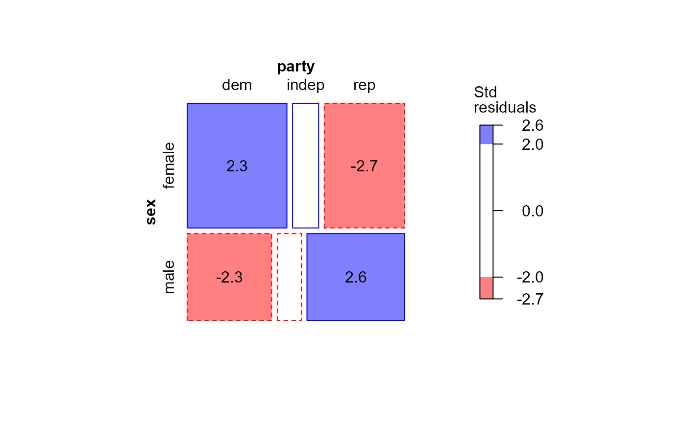
#> msc.gl> GSStab <- xtabs(count ~ sex + party, data=GSS)
#>
#> msc.gl> # using the data in table form
#> msc.gl> mod.glm1 <- glm(Freq ~ sex + party, family = poisson, data = GSStab)
#>
#> msc.gl> res <- residuals(mod.glm1)
#>
#> msc.gl> std <- rstandard(mod.glm1)
#>
#> msc.gl> # For mosaic.default(), need to re-shape residuals to conform to data
#> msc.gl> stdtab <- array(std,
#> msc.gl+ dim=dim(GSStab),
#> msc.gl+ dimnames=dimnames(GSStab))
#>
#> msc.gl> mosaic(GSStab,
#> msc.gl+ gp=shading_Friendly,
#> msc.gl+ residuals=stdtab,
#> msc.gl+ residuals_type="Std\nresiduals",
#> msc.gl+ labeling = labeling_residuals)
 #>
#> msc.gl> # Using externally calculated residuals with the glm() object
#> msc.gl> mosaic(mod.glm1,
#> msc.gl+ residuals=std,
#> msc.gl+ labeling = labeling_residuals,
#> msc.gl+ shade=TRUE)
#>
#> msc.gl> # Using externally calculated residuals with the glm() object
#> msc.gl> mosaic(mod.glm1,
#> msc.gl+ residuals=std,
#> msc.gl+ labeling = labeling_residuals,
#> msc.gl+ shade=TRUE)
 #>
#> msc.gl> # Using residuals_type
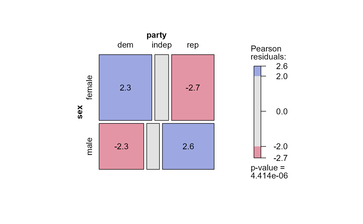
#> msc.gl> mosaic(mod.glm1,
#> msc.gl+ residuals_type="rstandard",
#> msc.gl+ labeling = labeling_residuals, shade=TRUE)
#>
#> msc.gl> # Using residuals_type
#> msc.gl> mosaic(mod.glm1,
#> msc.gl+ residuals_type="rstandard",
#> msc.gl+ labeling = labeling_residuals, shade=TRUE)
 #>
#> msc.gl> ## Ordinal factors and structured associations
#> msc.gl> data(Mental)
#>
#> msc.gl> xtabs(Freq ~ mental+ses, data=Mental)
#> ses
#> mental 1 2 3 4 5 6
#> Well 64 57 57 72 36 21
#> Mild 94 94 105 141 97 71
#> Moderate 58 54 65 77 54 54
#> Impaired 46 40 60 94 78 71
#>
#> msc.gl> long.labels <- list(set_varnames = c(mental="Mental Health Status",
#> msc.gl+ ses="Parent SES"))
#>
#> msc.gl> # fit independence model
#> msc.gl> # Residual deviance: 47.418 on 15 degrees of freedom
#> msc.gl> indep <- glm(Freq ~ mental+ses,
#> msc.gl+ family = poisson, data = Mental)
#>
#> msc.gl> long.labels <- list(set_varnames = c(mental="Mental Health Status",
#> msc.gl+ ses="Parent SES"))
#>
#> msc.gl> mosaic(indep,
#> msc.gl+ formula = ~ses + mental,
#> msc.gl+ residuals_type="rstandard",
#> msc.gl+ labeling_args = long.labels,
#> msc.gl+ labeling=labeling_residuals)
#>
#> msc.gl> ## Ordinal factors and structured associations
#> msc.gl> data(Mental)
#>
#> msc.gl> xtabs(Freq ~ mental+ses, data=Mental)
#> ses
#> mental 1 2 3 4 5 6
#> Well 64 57 57 72 36 21
#> Mild 94 94 105 141 97 71
#> Moderate 58 54 65 77 54 54
#> Impaired 46 40 60 94 78 71
#>
#> msc.gl> long.labels <- list(set_varnames = c(mental="Mental Health Status",
#> msc.gl+ ses="Parent SES"))
#>
#> msc.gl> # fit independence model
#> msc.gl> # Residual deviance: 47.418 on 15 degrees of freedom
#> msc.gl> indep <- glm(Freq ~ mental+ses,
#> msc.gl+ family = poisson, data = Mental)
#>
#> msc.gl> long.labels <- list(set_varnames = c(mental="Mental Health Status",
#> msc.gl+ ses="Parent SES"))
#>
#> msc.gl> mosaic(indep,
#> msc.gl+ formula = ~ses + mental,
#> msc.gl+ residuals_type="rstandard",
#> msc.gl+ labeling_args = long.labels,
#> msc.gl+ labeling=labeling_residuals)
 #>
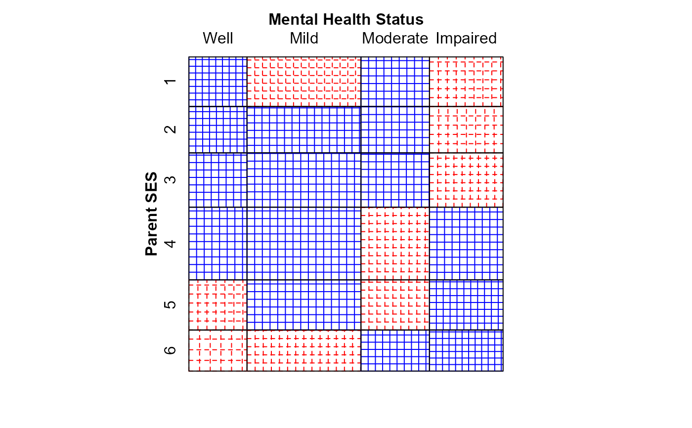
#> msc.gl> # or, show as a sieve diagram
#> msc.gl> mosaic(indep,
#> msc.gl+ formula = ~ses + mental,
#> msc.gl+ labeling_args = long.labels,
#> msc.gl+ panel=sieve,
#> msc.gl+ gp=shading_Friendly)
#>
#> msc.gl> # or, show as a sieve diagram
#> msc.gl> mosaic(indep,
#> msc.gl+ formula = ~ses + mental,
#> msc.gl+ labeling_args = long.labels,
#> msc.gl+ panel=sieve,
#> msc.gl+ gp=shading_Friendly)
 #>
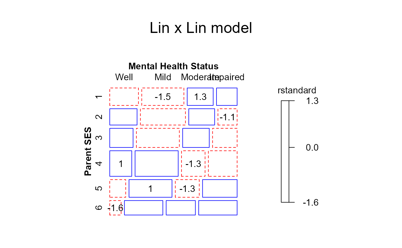
#> msc.gl> # fit linear x linear (uniform) association. Use integer scores for rows/cols
#> msc.gl> Cscore <- as.numeric(Mental$ses)
#>
#> msc.gl> Rscore <- as.numeric(Mental$mental)
#>
#> msc.gl> linlin <- glm(Freq ~ mental + ses + Rscore:Cscore,
#> msc.gl+ family = poisson, data = Mental)
#>
#> msc.gl> mosaic(linlin,
#> msc.gl+ formula = ~ses + mental,
#> msc.gl+ residuals_type="rstandard",
#> msc.gl+ labeling_args = long.labels,
#> msc.gl+ labeling=labeling_residuals,
#> msc.gl+ suppress=1,
#> msc.gl+ gp=shading_Friendly,
#> msc.gl+ main="Lin x Lin model")
#>
#> msc.gl> # fit linear x linear (uniform) association. Use integer scores for rows/cols
#> msc.gl> Cscore <- as.numeric(Mental$ses)
#>
#> msc.gl> Rscore <- as.numeric(Mental$mental)
#>
#> msc.gl> linlin <- glm(Freq ~ mental + ses + Rscore:Cscore,
#> msc.gl+ family = poisson, data = Mental)
#>
#> msc.gl> mosaic(linlin,
#> msc.gl+ formula = ~ses + mental,
#> msc.gl+ residuals_type="rstandard",
#> msc.gl+ labeling_args = long.labels,
#> msc.gl+ labeling=labeling_residuals,
#> msc.gl+ suppress=1,
#> msc.gl+ gp=shading_Friendly,
#> msc.gl+ main="Lin x Lin model")
 #>
#> msc.gl> ## Goodman Row-Column association model fits even better (deviance 3.57, df 8)
#> msc.gl> if (require(gnm)) {
#> msc.gl+ Mental$mental <- C(Mental$mental, treatment)
#> msc.gl+ Mental$ses <- C(Mental$ses, treatment)
#> msc.gl+ RC1model <- gnm(Freq ~ ses + mental + Mult(ses, mental),
#> msc.gl+ family = poisson, data = Mental)
#> msc.gl+
#> msc.gl+ mosaic(RC1model,
#> msc.gl+ formula = ~ses + mental,
#> msc.gl+ residuals_type="rstandard",
#> msc.gl+ labeling_args = long.labels,
#> msc.gl+ labeling=labeling_residuals,
#> msc.gl+ suppress=1,
#> msc.gl+ gp=shading_Friendly,
#> msc.gl+ main="RC1 model")
#> msc.gl+ }
#> Initialising
#> Running start-up iterations..
#> Running main iterations........
#> Done
#>
#> msc.gl> ## Goodman Row-Column association model fits even better (deviance 3.57, df 8)
#> msc.gl> if (require(gnm)) {
#> msc.gl+ Mental$mental <- C(Mental$mental, treatment)
#> msc.gl+ Mental$ses <- C(Mental$ses, treatment)
#> msc.gl+ RC1model <- gnm(Freq ~ ses + mental + Mult(ses, mental),
#> msc.gl+ family = poisson, data = Mental)
#> msc.gl+
#> msc.gl+ mosaic(RC1model,
#> msc.gl+ formula = ~ses + mental,
#> msc.gl+ residuals_type="rstandard",
#> msc.gl+ labeling_args = long.labels,
#> msc.gl+ labeling=labeling_residuals,
#> msc.gl+ suppress=1,
#> msc.gl+ gp=shading_Friendly,
#> msc.gl+ main="RC1 model")
#> msc.gl+ }
#> Initialising
#> Running start-up iterations..
#> Running main iterations........
#> Done
 #>
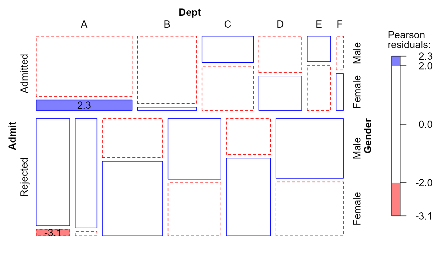
#> msc.gl> ############# UCB Admissions data, fit using glm()
#> msc.gl>
#> msc.gl> structable(Dept ~ Admit+Gender,UCBAdmissions)
#> Dept A B C D E F
#> Admit Gender
#> Admitted Male 512 353 120 138 53 22
#> Female 89 17 202 131 94 24
#> Rejected Male 313 207 205 279 138 351
#> Female 19 8 391 244 299 317
#>
#> msc.gl> berkeley <- as.data.frame(UCBAdmissions)
#>
#> msc.gl> berk.glm1 <- glm(Freq ~ Dept * (Gender+Admit), data=berkeley, family="poisson")
#>
#> msc.gl> summary(berk.glm1)
#>
#> Call:
#> glm(formula = Freq ~ Dept * (Gender + Admit), family = "poisson",
#> data = berkeley)
#>
#> Coefficients:
#> Estimate Std. Error z value Pr(>|z|)
#> (Intercept) 6.27557 0.04248 147.744 < 2e-16 ***
#> DeptB -0.40575 0.06770 -5.993 2.06e-09 ***
#> DeptC -1.53939 0.08305 -18.536 < 2e-16 ***
#> DeptD -1.32234 0.08159 -16.207 < 2e-16 ***
#> DeptE -2.40277 0.11014 -21.816 < 2e-16 ***
#> DeptF -3.09624 0.15756 -19.652 < 2e-16 ***
#> GenderFemale -2.03325 0.10233 -19.870 < 2e-16 ***
#> AdmitRejected -0.59346 0.06838 -8.679 < 2e-16 ***
#> DeptB:GenderFemale -1.07581 0.22860 -4.706 2.52e-06 ***
#> DeptC:GenderFemale 2.63462 0.12343 21.345 < 2e-16 ***
#> DeptD:GenderFemale 1.92709 0.12464 15.461 < 2e-16 ***
#> DeptE:GenderFemale 2.75479 0.13510 20.391 < 2e-16 ***
#> DeptF:GenderFemale 1.94356 0.12683 15.325 < 2e-16 ***
#> DeptB:AdmitRejected 0.05059 0.10968 0.461 0.645
#> DeptC:AdmitRejected 1.20915 0.09726 12.432 < 2e-16 ***
#> DeptD:AdmitRejected 1.25833 0.10152 12.395 < 2e-16 ***
#> DeptE:AdmitRejected 1.68296 0.11733 14.343 < 2e-16 ***
#> DeptF:AdmitRejected 3.26911 0.16707 19.567 < 2e-16 ***
#> ---
#> Signif. codes: 0 ‘***’ 0.001 ‘**’ 0.01 ‘*’ 0.05 ‘.’ 0.1 ‘ ’ 1
#>
#> (Dispersion parameter for poisson family taken to be 1)
#>
#> Null deviance: 2650.095 on 23 degrees of freedom
#> Residual deviance: 21.736 on 6 degrees of freedom
#> AIC: 216.8
#>
#> Number of Fisher Scoring iterations: 4
#>
#>
#> msc.gl> mosaic(berk.glm1,
#> msc.gl+ gp=shading_Friendly,
#> msc.gl+ labeling=labeling_residuals,
#> msc.gl+ formula=~Admit+Dept+Gender)
#>
#> msc.gl> ############# UCB Admissions data, fit using glm()
#> msc.gl>
#> msc.gl> structable(Dept ~ Admit+Gender,UCBAdmissions)
#> Dept A B C D E F
#> Admit Gender
#> Admitted Male 512 353 120 138 53 22
#> Female 89 17 202 131 94 24
#> Rejected Male 313 207 205 279 138 351
#> Female 19 8 391 244 299 317
#>
#> msc.gl> berkeley <- as.data.frame(UCBAdmissions)
#>
#> msc.gl> berk.glm1 <- glm(Freq ~ Dept * (Gender+Admit), data=berkeley, family="poisson")
#>
#> msc.gl> summary(berk.glm1)
#>
#> Call:
#> glm(formula = Freq ~ Dept * (Gender + Admit), family = "poisson",
#> data = berkeley)
#>
#> Coefficients:
#> Estimate Std. Error z value Pr(>|z|)
#> (Intercept) 6.27557 0.04248 147.744 < 2e-16 ***
#> DeptB -0.40575 0.06770 -5.993 2.06e-09 ***
#> DeptC -1.53939 0.08305 -18.536 < 2e-16 ***
#> DeptD -1.32234 0.08159 -16.207 < 2e-16 ***
#> DeptE -2.40277 0.11014 -21.816 < 2e-16 ***
#> DeptF -3.09624 0.15756 -19.652 < 2e-16 ***
#> GenderFemale -2.03325 0.10233 -19.870 < 2e-16 ***
#> AdmitRejected -0.59346 0.06838 -8.679 < 2e-16 ***
#> DeptB:GenderFemale -1.07581 0.22860 -4.706 2.52e-06 ***
#> DeptC:GenderFemale 2.63462 0.12343 21.345 < 2e-16 ***
#> DeptD:GenderFemale 1.92709 0.12464 15.461 < 2e-16 ***
#> DeptE:GenderFemale 2.75479 0.13510 20.391 < 2e-16 ***
#> DeptF:GenderFemale 1.94356 0.12683 15.325 < 2e-16 ***
#> DeptB:AdmitRejected 0.05059 0.10968 0.461 0.645
#> DeptC:AdmitRejected 1.20915 0.09726 12.432 < 2e-16 ***
#> DeptD:AdmitRejected 1.25833 0.10152 12.395 < 2e-16 ***
#> DeptE:AdmitRejected 1.68296 0.11733 14.343 < 2e-16 ***
#> DeptF:AdmitRejected 3.26911 0.16707 19.567 < 2e-16 ***
#> ---
#> Signif. codes: 0 ‘***’ 0.001 ‘**’ 0.01 ‘*’ 0.05 ‘.’ 0.1 ‘ ’ 1
#>
#> (Dispersion parameter for poisson family taken to be 1)
#>
#> Null deviance: 2650.095 on 23 degrees of freedom
#> Residual deviance: 21.736 on 6 degrees of freedom
#> AIC: 216.8
#>
#> Number of Fisher Scoring iterations: 4
#>
#>
#> msc.gl> mosaic(berk.glm1,
#> msc.gl+ gp=shading_Friendly,
#> msc.gl+ labeling=labeling_residuals,
#> msc.gl+ formula=~Admit+Dept+Gender)
 #>
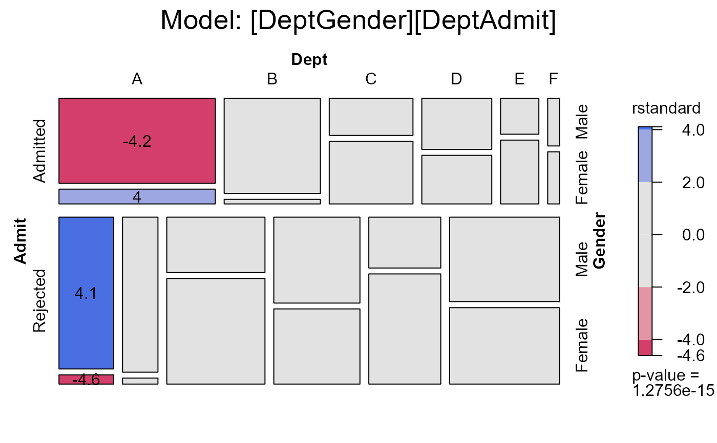
#> msc.gl> # the same, displaying studentized residuals;
#> msc.gl> # note use of formula to reorder factors in the mosaic
#> msc.gl> mosaic(berk.glm1,
#> msc.gl+ residuals_type="rstandard",
#> msc.gl+ labeling=labeling_residuals,
#> msc.gl+ shade=TRUE,
#> msc.gl+ formula=~Admit+Dept+Gender,
#> msc.gl+ main="Model: [DeptGender][DeptAdmit]")
#>
#> msc.gl> # the same, displaying studentized residuals;
#> msc.gl> # note use of formula to reorder factors in the mosaic
#> msc.gl> mosaic(berk.glm1,
#> msc.gl+ residuals_type="rstandard",
#> msc.gl+ labeling=labeling_residuals,
#> msc.gl+ shade=TRUE,
#> msc.gl+ formula=~Admit+Dept+Gender,
#> msc.gl+ main="Model: [DeptGender][DeptAdmit]")
 #>
#> msc.gl> ## all two-way model
#> msc.gl> berk.glm2 <- glm(Freq ~ (Dept + Gender + Admit)^2, data=berkeley, family="poisson")
#>
#> msc.gl> summary(berk.glm2)
#>
#> Call:
#> glm(formula = Freq ~ (Dept + Gender + Admit)^2, family = "poisson",
#> data = berkeley)
#>
#> Coefficients:
#> Estimate Std. Error z value Pr(>|z|)
#> (Intercept) 6.27150 0.04271 146.855 < 2e-16 ***
#> DeptB -0.40322 0.06784 -5.944 2.78e-09 ***
#> DeptC -1.57790 0.08949 -17.632 < 2e-16 ***
#> DeptD -1.35000 0.08526 -15.834 < 2e-16 ***
#> DeptE -2.44982 0.11755 -20.840 < 2e-16 ***
#> DeptF -3.13787 0.16174 -19.401 < 2e-16 ***
#> GenderFemale -1.99859 0.10593 -18.866 < 2e-16 ***
#> AdmitRejected -0.58205 0.06899 -8.436 < 2e-16 ***
#> DeptB:GenderFemale -1.07482 0.22861 -4.701 2.58e-06 ***
#> DeptC:GenderFemale 2.66513 0.12609 21.137 < 2e-16 ***
#> DeptD:GenderFemale 1.95832 0.12734 15.379 < 2e-16 ***
#> DeptE:GenderFemale 2.79519 0.13925 20.073 < 2e-16 ***
#> DeptF:GenderFemale 2.00232 0.13571 14.754 < 2e-16 ***
#> DeptB:AdmitRejected 0.04340 0.10984 0.395 0.693
#> DeptC:AdmitRejected 1.26260 0.10663 11.841 < 2e-16 ***
#> DeptD:AdmitRejected 1.29461 0.10582 12.234 < 2e-16 ***
#> DeptE:AdmitRejected 1.73931 0.12611 13.792 < 2e-16 ***
#> DeptF:AdmitRejected 3.30648 0.16998 19.452 < 2e-16 ***
#> GenderFemale:AdmitRejected -0.09987 0.08085 -1.235 0.217
#> ---
#> Signif. codes: 0 ‘***’ 0.001 ‘**’ 0.01 ‘*’ 0.05 ‘.’ 0.1 ‘ ’ 1
#>
#> (Dispersion parameter for poisson family taken to be 1)
#>
#> Null deviance: 2650.095 on 23 degrees of freedom
#> Residual deviance: 20.204 on 5 degrees of freedom
#> AIC: 217.26
#>
#> Number of Fisher Scoring iterations: 4
#>
#>
#> msc.gl> mosaic(berk.glm2,
#> msc.gl+ residuals_type="rstandard",
#> msc.gl+ labeling = labeling_residuals,
#> msc.gl+ shade=TRUE,
#> msc.gl+ formula=~Admit+Dept+Gender,
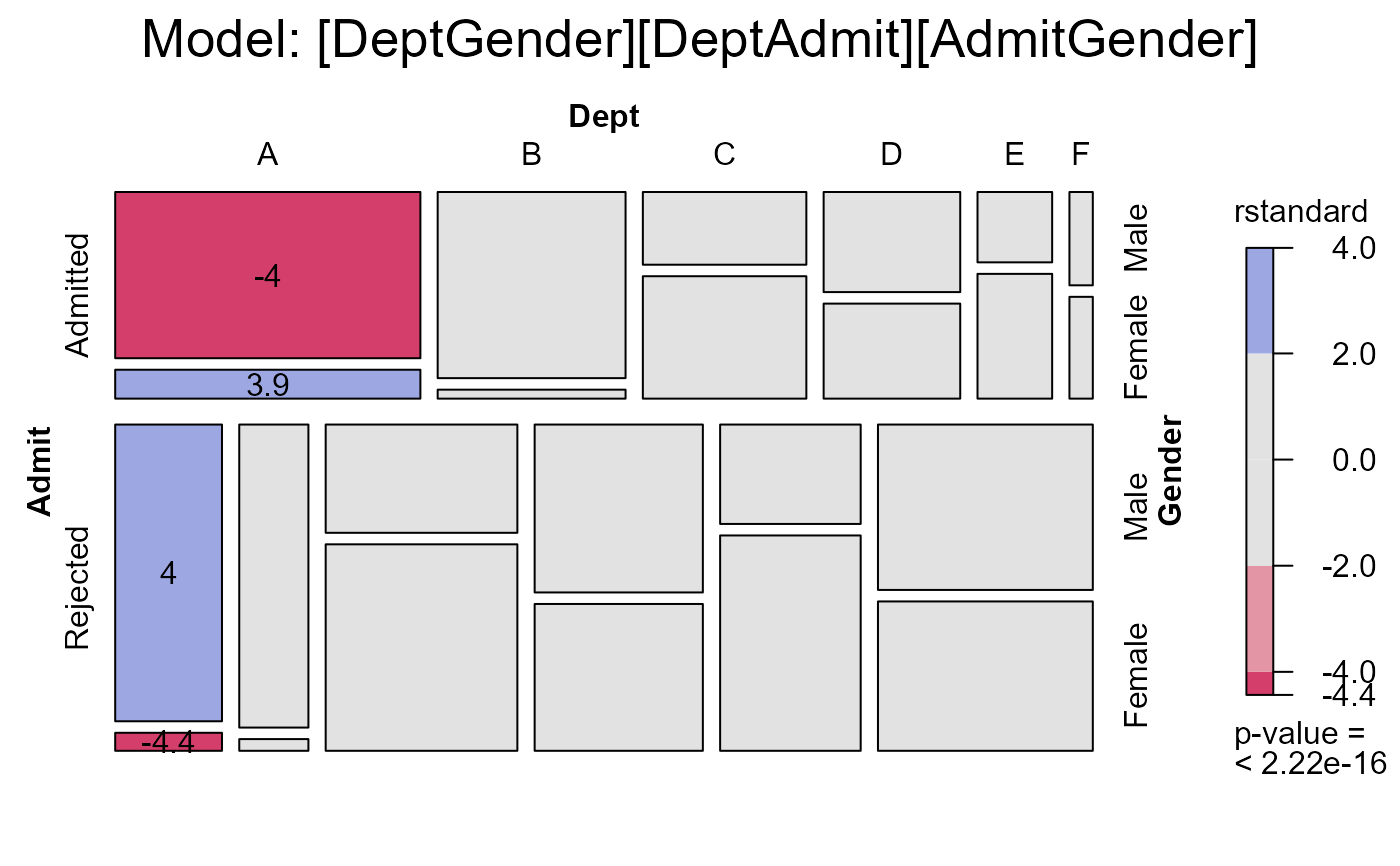
#> msc.gl+ main="Model: [DeptGender][DeptAdmit][AdmitGender]")
#>
#> msc.gl> ## all two-way model
#> msc.gl> berk.glm2 <- glm(Freq ~ (Dept + Gender + Admit)^2, data=berkeley, family="poisson")
#>
#> msc.gl> summary(berk.glm2)
#>
#> Call:
#> glm(formula = Freq ~ (Dept + Gender + Admit)^2, family = "poisson",
#> data = berkeley)
#>
#> Coefficients:
#> Estimate Std. Error z value Pr(>|z|)
#> (Intercept) 6.27150 0.04271 146.855 < 2e-16 ***
#> DeptB -0.40322 0.06784 -5.944 2.78e-09 ***
#> DeptC -1.57790 0.08949 -17.632 < 2e-16 ***
#> DeptD -1.35000 0.08526 -15.834 < 2e-16 ***
#> DeptE -2.44982 0.11755 -20.840 < 2e-16 ***
#> DeptF -3.13787 0.16174 -19.401 < 2e-16 ***
#> GenderFemale -1.99859 0.10593 -18.866 < 2e-16 ***
#> AdmitRejected -0.58205 0.06899 -8.436 < 2e-16 ***
#> DeptB:GenderFemale -1.07482 0.22861 -4.701 2.58e-06 ***
#> DeptC:GenderFemale 2.66513 0.12609 21.137 < 2e-16 ***
#> DeptD:GenderFemale 1.95832 0.12734 15.379 < 2e-16 ***
#> DeptE:GenderFemale 2.79519 0.13925 20.073 < 2e-16 ***
#> DeptF:GenderFemale 2.00232 0.13571 14.754 < 2e-16 ***
#> DeptB:AdmitRejected 0.04340 0.10984 0.395 0.693
#> DeptC:AdmitRejected 1.26260 0.10663 11.841 < 2e-16 ***
#> DeptD:AdmitRejected 1.29461 0.10582 12.234 < 2e-16 ***
#> DeptE:AdmitRejected 1.73931 0.12611 13.792 < 2e-16 ***
#> DeptF:AdmitRejected 3.30648 0.16998 19.452 < 2e-16 ***
#> GenderFemale:AdmitRejected -0.09987 0.08085 -1.235 0.217
#> ---
#> Signif. codes: 0 ‘***’ 0.001 ‘**’ 0.01 ‘*’ 0.05 ‘.’ 0.1 ‘ ’ 1
#>
#> (Dispersion parameter for poisson family taken to be 1)
#>
#> Null deviance: 2650.095 on 23 degrees of freedom
#> Residual deviance: 20.204 on 5 degrees of freedom
#> AIC: 217.26
#>
#> Number of Fisher Scoring iterations: 4
#>
#>
#> msc.gl> mosaic(berk.glm2,
#> msc.gl+ residuals_type="rstandard",
#> msc.gl+ labeling = labeling_residuals,
#> msc.gl+ shade=TRUE,
#> msc.gl+ formula=~Admit+Dept+Gender,
#> msc.gl+ main="Model: [DeptGender][DeptAdmit][AdmitGender]")
 #>
#> msc.gl> anova(berk.glm1, berk.glm2, test="Chisq")
#> Analysis of Deviance Table
#>
#> Model 1: Freq ~ Dept * (Gender + Admit)
#> Model 2: Freq ~ (Dept + Gender + Admit)^2
#> Resid. Df Resid. Dev Df Deviance Pr(>Chi)
#> 1 6 21.735
#> 2 5 20.204 1 1.5312 0.2159
#>
#> msc.gl> # Add 1 df term for association of [GenderAdmit] only in Dept A
#> msc.gl> berkeley <- within(berkeley,
#> msc.gl+ dept1AG <- (Dept=='A')*(Gender=='Female')*(Admit=='Admitted'))
#>
#> msc.gl> berkeley[1:6,]
#> Admit Gender Dept Freq dept1AG
#> 1 Admitted Male A 512 0
#> 2 Rejected Male A 313 0
#> 3 Admitted Female A 89 1
#> 4 Rejected Female A 19 0
#> 5 Admitted Male B 353 0
#> 6 Rejected Male B 207 0
#>
#> msc.gl> berk.glm3 <- glm(Freq ~ Dept * (Gender+Admit) + dept1AG, data=berkeley, family="poisson")
#>
#> msc.gl> summary(berk.glm3)
#>
#> Call:
#> glm(formula = Freq ~ Dept * (Gender + Admit) + dept1AG, family = "poisson",
#> data = berkeley)
#>
#> Coefficients:
#> Estimate Std. Error z value Pr(>|z|)
#> (Intercept) 6.23832 0.04419 141.157 < 2e-16 ***
#> DeptB -0.36850 0.06879 -5.357 8.47e-08 ***
#> DeptC -1.50215 0.08394 -17.895 < 2e-16 ***
#> DeptD -1.28509 0.08250 -15.577 < 2e-16 ***
#> DeptE -2.36552 0.11081 -21.347 < 2e-16 ***
#> DeptF -3.05899 0.15803 -19.357 < 2e-16 ***
#> GenderFemale -2.80176 0.23628 -11.858 < 2e-16 ***
#> AdmitRejected -0.49212 0.07175 -6.859 6.94e-12 ***
#> dept1AG 1.05208 0.26271 4.005 6.21e-05 ***
#> DeptB:GenderFemale -0.30730 0.31243 -0.984 0.325
#> DeptC:GenderFemale 3.40313 0.24615 13.825 < 2e-16 ***
#> DeptD:GenderFemale 2.69560 0.24676 10.924 < 2e-16 ***
#> DeptE:GenderFemale 3.52330 0.25220 13.970 < 2e-16 ***
#> DeptF:GenderFemale 2.71207 0.24787 10.941 < 2e-16 ***
#> DeptB:AdmitRejected -0.05074 0.11181 -0.454 0.650
#> DeptC:AdmitRejected 1.10781 0.09966 11.116 < 2e-16 ***
#> DeptD:AdmitRejected 1.15699 0.10381 11.145 < 2e-16 ***
#> DeptE:AdmitRejected 1.58162 0.11933 13.254 < 2e-16 ***
#> DeptF:AdmitRejected 3.16777 0.16848 18.803 < 2e-16 ***
#> ---
#> Signif. codes: 0 ‘***’ 0.001 ‘**’ 0.01 ‘*’ 0.05 ‘.’ 0.1 ‘ ’ 1
#>
#> (Dispersion parameter for poisson family taken to be 1)
#>
#> Null deviance: 2650.0952 on 23 degrees of freedom
#> Residual deviance: 2.6815 on 5 degrees of freedom
#> AIC: 199.74
#>
#> Number of Fisher Scoring iterations: 3
#>
#>
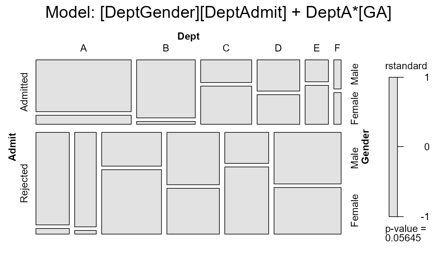
#> msc.gl> mosaic(berk.glm3,
#> msc.gl+ residuals_type = "rstandard",
#> msc.gl+ labeling = labeling_residuals,
#> msc.gl+ shade=TRUE,
#> msc.gl+ formula = ~Admit+Dept+Gender,
#> msc.gl+ main = "Model: [DeptGender][DeptAdmit] + DeptA*[GA]")
#>
#> msc.gl> anova(berk.glm1, berk.glm2, test="Chisq")
#> Analysis of Deviance Table
#>
#> Model 1: Freq ~ Dept * (Gender + Admit)
#> Model 2: Freq ~ (Dept + Gender + Admit)^2
#> Resid. Df Resid. Dev Df Deviance Pr(>Chi)
#> 1 6 21.735
#> 2 5 20.204 1 1.5312 0.2159
#>
#> msc.gl> # Add 1 df term for association of [GenderAdmit] only in Dept A
#> msc.gl> berkeley <- within(berkeley,
#> msc.gl+ dept1AG <- (Dept=='A')*(Gender=='Female')*(Admit=='Admitted'))
#>
#> msc.gl> berkeley[1:6,]
#> Admit Gender Dept Freq dept1AG
#> 1 Admitted Male A 512 0
#> 2 Rejected Male A 313 0
#> 3 Admitted Female A 89 1
#> 4 Rejected Female A 19 0
#> 5 Admitted Male B 353 0
#> 6 Rejected Male B 207 0
#>
#> msc.gl> berk.glm3 <- glm(Freq ~ Dept * (Gender+Admit) + dept1AG, data=berkeley, family="poisson")
#>
#> msc.gl> summary(berk.glm3)
#>
#> Call:
#> glm(formula = Freq ~ Dept * (Gender + Admit) + dept1AG, family = "poisson",
#> data = berkeley)
#>
#> Coefficients:
#> Estimate Std. Error z value Pr(>|z|)
#> (Intercept) 6.23832 0.04419 141.157 < 2e-16 ***
#> DeptB -0.36850 0.06879 -5.357 8.47e-08 ***
#> DeptC -1.50215 0.08394 -17.895 < 2e-16 ***
#> DeptD -1.28509 0.08250 -15.577 < 2e-16 ***
#> DeptE -2.36552 0.11081 -21.347 < 2e-16 ***
#> DeptF -3.05899 0.15803 -19.357 < 2e-16 ***
#> GenderFemale -2.80176 0.23628 -11.858 < 2e-16 ***
#> AdmitRejected -0.49212 0.07175 -6.859 6.94e-12 ***
#> dept1AG 1.05208 0.26271 4.005 6.21e-05 ***
#> DeptB:GenderFemale -0.30730 0.31243 -0.984 0.325
#> DeptC:GenderFemale 3.40313 0.24615 13.825 < 2e-16 ***
#> DeptD:GenderFemale 2.69560 0.24676 10.924 < 2e-16 ***
#> DeptE:GenderFemale 3.52330 0.25220 13.970 < 2e-16 ***
#> DeptF:GenderFemale 2.71207 0.24787 10.941 < 2e-16 ***
#> DeptB:AdmitRejected -0.05074 0.11181 -0.454 0.650
#> DeptC:AdmitRejected 1.10781 0.09966 11.116 < 2e-16 ***
#> DeptD:AdmitRejected 1.15699 0.10381 11.145 < 2e-16 ***
#> DeptE:AdmitRejected 1.58162 0.11933 13.254 < 2e-16 ***
#> DeptF:AdmitRejected 3.16777 0.16848 18.803 < 2e-16 ***
#> ---
#> Signif. codes: 0 ‘***’ 0.001 ‘**’ 0.01 ‘*’ 0.05 ‘.’ 0.1 ‘ ’ 1
#>
#> (Dispersion parameter for poisson family taken to be 1)
#>
#> Null deviance: 2650.0952 on 23 degrees of freedom
#> Residual deviance: 2.6815 on 5 degrees of freedom
#> AIC: 199.74
#>
#> Number of Fisher Scoring iterations: 3
#>
#>
#> msc.gl> mosaic(berk.glm3,
#> msc.gl+ residuals_type = "rstandard",
#> msc.gl+ labeling = labeling_residuals,
#> msc.gl+ shade=TRUE,
#> msc.gl+ formula = ~Admit+Dept+Gender,
#> msc.gl+ main = "Model: [DeptGender][DeptAdmit] + DeptA*[GA]")
 #>
#> msc.gl> # compare models
#> msc.gl> anova(berk.glm1, berk.glm3, test="Chisq")
#> Analysis of Deviance Table
#>
#> Model 1: Freq ~ Dept * (Gender + Admit)
#> Model 2: Freq ~ Dept * (Gender + Admit) + dept1AG
#> Resid. Df Resid. Dev Df Deviance Pr(>Chi)
#> 1 6 21.7355
#> 2 5 2.6815 1 19.054 1.271e-05 ***
#> ---
#> Signif. codes: 0 ‘***’ 0.001 ‘**’ 0.01 ‘*’ 0.05 ‘.’ 0.1 ‘ ’ 1
demo("mental-glm")
#>
#>
#> demo(mental-glm)
#> ---- ~~~~~~~~~~
#>
#> > ## Mental health data: mosaics for glm() and gnm() models
#> > library(gnm)
#>
#> > library(vcdExtra)
#>
#> > data(Mental)
#>
#> > # display the frequency table
#> > (Mental.tab <- xtabs(Freq ~ mental+ses, data=Mental))
#> ses
#> mental 1 2 3 4 5 6
#> Well 64 57 57 72 36 21
#> Mild 94 94 105 141 97 71
#> Moderate 58 54 65 77 54 54
#> Impaired 46 40 60 94 78 71
#>
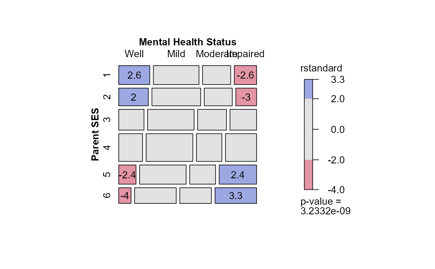
#> > # fit independence model
#> > # Residual deviance: 47.418 on 15 degrees of freedom
#> > indep <- glm(Freq ~ mental+ses,
#> + family = poisson, data = Mental)
#>
#> > deviance(indep)
#> [1] 47.41785
#>
#> > long.labels <- list(set_varnames = c(mental="Mental Health Status", ses="Parent SES"))
#>
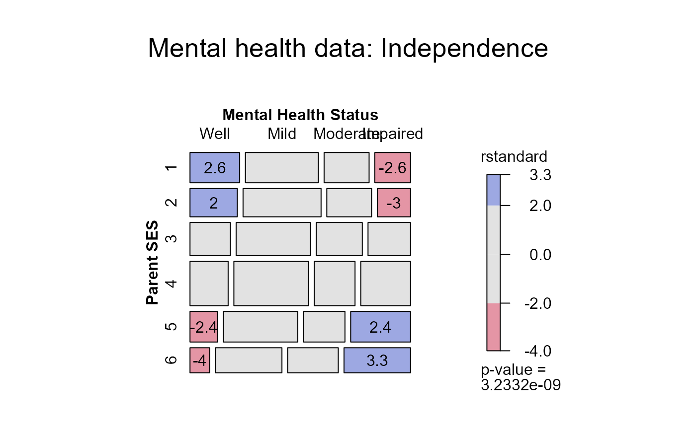
#> > mosaic(indep,residuals_type="rstandard", labeling_args = long.labels, labeling=labeling_residuals,
#> + main="Mental health data: Independence")
#> Warning: no formula provided, assuming ~ses + mental
#>
#> msc.gl> # compare models
#> msc.gl> anova(berk.glm1, berk.glm3, test="Chisq")
#> Analysis of Deviance Table
#>
#> Model 1: Freq ~ Dept * (Gender + Admit)
#> Model 2: Freq ~ Dept * (Gender + Admit) + dept1AG
#> Resid. Df Resid. Dev Df Deviance Pr(>Chi)
#> 1 6 21.7355
#> 2 5 2.6815 1 19.054 1.271e-05 ***
#> ---
#> Signif. codes: 0 ‘***’ 0.001 ‘**’ 0.01 ‘*’ 0.05 ‘.’ 0.1 ‘ ’ 1
demo("mental-glm")
#>
#>
#> demo(mental-glm)
#> ---- ~~~~~~~~~~
#>
#> > ## Mental health data: mosaics for glm() and gnm() models
#> > library(gnm)
#>
#> > library(vcdExtra)
#>
#> > data(Mental)
#>
#> > # display the frequency table
#> > (Mental.tab <- xtabs(Freq ~ mental+ses, data=Mental))
#> ses
#> mental 1 2 3 4 5 6
#> Well 64 57 57 72 36 21
#> Mild 94 94 105 141 97 71
#> Moderate 58 54 65 77 54 54
#> Impaired 46 40 60 94 78 71
#>
#> > # fit independence model
#> > # Residual deviance: 47.418 on 15 degrees of freedom
#> > indep <- glm(Freq ~ mental+ses,
#> + family = poisson, data = Mental)
#>
#> > deviance(indep)
#> [1] 47.41785
#>
#> > long.labels <- list(set_varnames = c(mental="Mental Health Status", ses="Parent SES"))
#>
#> > mosaic(indep,residuals_type="rstandard", labeling_args = long.labels, labeling=labeling_residuals,
#> + main="Mental health data: Independence")
#> Warning: no formula provided, assuming ~ses + mental
 #>
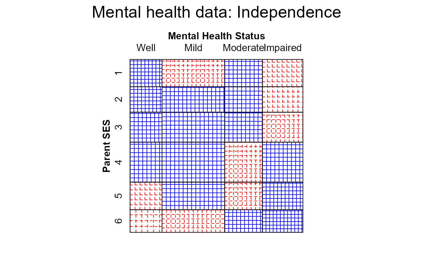
#> > # as a sieve diagram
#> > mosaic(indep, labeling_args = long.labels, panel=sieve, gp=shading_Friendly,
#> + main="Mental health data: Independence")
#> Warning: no formula provided, assuming ~ses + mental
#>
#> > # as a sieve diagram
#> > mosaic(indep, labeling_args = long.labels, panel=sieve, gp=shading_Friendly,
#> + main="Mental health data: Independence")
#> Warning: no formula provided, assuming ~ses + mental
 #>
#> > # fit linear x linear (uniform) association. Use integer scores for rows/cols
#> > Cscore <- as.numeric(Mental$ses)
#>
#> > Rscore <- as.numeric(Mental$mental)
#>
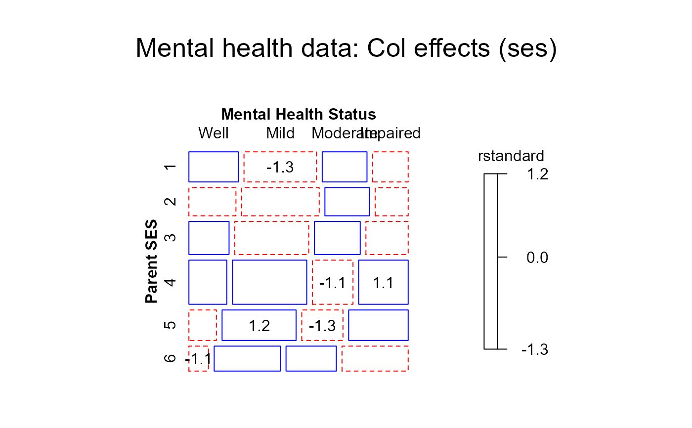
#> > # column effects model (ses)
#> > coleff <- glm(Freq ~ mental + ses + Rscore:ses,
#> + family = poisson, data = Mental)
#>
#> > mosaic(coleff,residuals_type="rstandard",
#> + labeling_args = long.labels, labeling=labeling_residuals, suppress=1, gp=shading_Friendly,
#> + main="Mental health data: Col effects (ses)")
#> Warning: no formula provided, assuming ~ses + mental
#>
#> > # fit linear x linear (uniform) association. Use integer scores for rows/cols
#> > Cscore <- as.numeric(Mental$ses)
#>
#> > Rscore <- as.numeric(Mental$mental)
#>
#> > # column effects model (ses)
#> > coleff <- glm(Freq ~ mental + ses + Rscore:ses,
#> + family = poisson, data = Mental)
#>
#> > mosaic(coleff,residuals_type="rstandard",
#> + labeling_args = long.labels, labeling=labeling_residuals, suppress=1, gp=shading_Friendly,
#> + main="Mental health data: Col effects (ses)")
#> Warning: no formula provided, assuming ~ses + mental
 #>
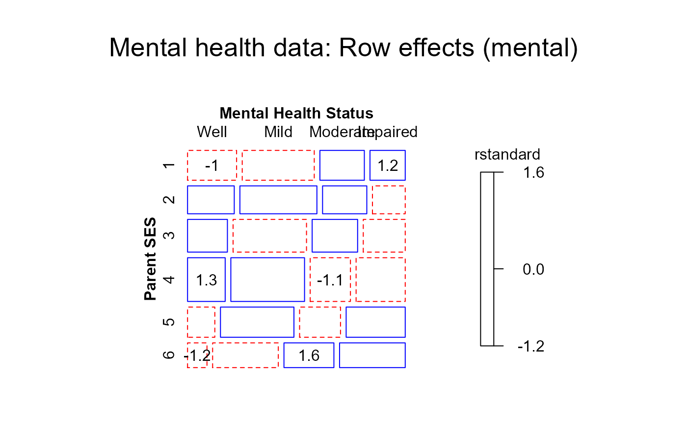
#> > # row effects model (mental)
#> > roweff <- glm(Freq ~ mental + ses + mental:Cscore,
#> + family = poisson, data = Mental)
#>
#> > mosaic(roweff,residuals_type="rstandard",
#> + labeling_args = long.labels, labeling=labeling_residuals, suppress=1, gp=shading_Friendly,
#> + main="Mental health data: Row effects (mental)")
#> Warning: no formula provided, assuming ~ses + mental
#>
#> > # row effects model (mental)
#> > roweff <- glm(Freq ~ mental + ses + mental:Cscore,
#> + family = poisson, data = Mental)
#>
#> > mosaic(roweff,residuals_type="rstandard",
#> + labeling_args = long.labels, labeling=labeling_residuals, suppress=1, gp=shading_Friendly,
#> + main="Mental health data: Row effects (mental)")
#> Warning: no formula provided, assuming ~ses + mental
 #>
#> > linlin <- glm(Freq ~ mental + ses + Rscore:Cscore,
#> + family = poisson, data = Mental)
#>
#> > # compare models
#> > anova(indep, roweff, coleff, linlin)
#> Analysis of Deviance Table
#>
#> Model 1: Freq ~ mental + ses
#> Model 2: Freq ~ mental + ses + mental:Cscore
#> Model 3: Freq ~ mental + ses + Rscore:ses
#> Model 4: Freq ~ mental + ses + Rscore:Cscore
#> Resid. Df Resid. Dev Df Deviance Pr(>Chi)
#> 1 15 47.418
#> 2 12 6.281 3 41.137 6.116e-09 ***
#> 3 10 6.829 2 -0.549
#> 4 14 9.895 -4 -3.066 0.5469
#> ---
#> Signif. codes: 0 ‘***’ 0.001 ‘**’ 0.01 ‘*’ 0.05 ‘.’ 0.1 ‘ ’ 1
#>
#> > AIC(indep, roweff, coleff, linlin)
#> df AIC
#> indep 9 209.5908
#> roweff 12 174.4537
#> coleff 14 179.0023
#> linlin 10 174.0681
#>
#> > mosaic(linlin,residuals_type="rstandard",
#> + labeling_args = long.labels, labeling=labeling_residuals, suppress=1, gp=shading_Friendly,
#> + main="Mental health data: Linear x Linear")
#> Warning: no formula provided, assuming ~ses + mental
#>
#> > linlin <- glm(Freq ~ mental + ses + Rscore:Cscore,
#> + family = poisson, data = Mental)
#>
#> > # compare models
#> > anova(indep, roweff, coleff, linlin)
#> Analysis of Deviance Table
#>
#> Model 1: Freq ~ mental + ses
#> Model 2: Freq ~ mental + ses + mental:Cscore
#> Model 3: Freq ~ mental + ses + Rscore:ses
#> Model 4: Freq ~ mental + ses + Rscore:Cscore
#> Resid. Df Resid. Dev Df Deviance Pr(>Chi)
#> 1 15 47.418
#> 2 12 6.281 3 41.137 6.116e-09 ***
#> 3 10 6.829 2 -0.549
#> 4 14 9.895 -4 -3.066 0.5469
#> ---
#> Signif. codes: 0 ‘***’ 0.001 ‘**’ 0.01 ‘*’ 0.05 ‘.’ 0.1 ‘ ’ 1
#>
#> > AIC(indep, roweff, coleff, linlin)
#> df AIC
#> indep 9 209.5908
#> roweff 12 174.4537
#> coleff 14 179.0023
#> linlin 10 174.0681
#>
#> > mosaic(linlin,residuals_type="rstandard",
#> + labeling_args = long.labels, labeling=labeling_residuals, suppress=1, gp=shading_Friendly,
#> + main="Mental health data: Linear x Linear")
#> Warning: no formula provided, assuming ~ses + mental
 #>
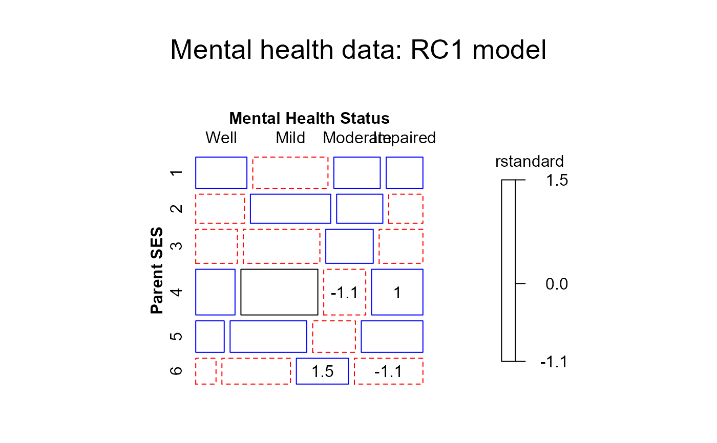
#> > ## Goodman Row-Column association model fits well (deviance 3.57, df 8)
#> > Mental$mental <- C(Mental$mental, treatment)
#>
#> > Mental$ses <- C(Mental$ses, treatment)
#>
#> > RC1model <- gnm(Freq ~ mental + ses + Mult(mental, ses),
#> + family = poisson, data = Mental)
#> Initialising
#> Running start-up iterations..
#> Running main iterations........
#> Done
#>
#> > mosaic(RC1model,residuals_type="rstandard",
#> + labeling_args = long.labels, labeling=labeling_residuals, suppress=1, gp=shading_Friendly,
#> + main="Mental health data: RC1 model")
#> Warning: no formula provided, assuming ~ses + mental
#>
#> > ## Goodman Row-Column association model fits well (deviance 3.57, df 8)
#> > Mental$mental <- C(Mental$mental, treatment)
#>
#> > Mental$ses <- C(Mental$ses, treatment)
#>
#> > RC1model <- gnm(Freq ~ mental + ses + Mult(mental, ses),
#> + family = poisson, data = Mental)
#> Initialising
#> Running start-up iterations..
#> Running main iterations........
#> Done
#>
#> > mosaic(RC1model,residuals_type="rstandard",
#> + labeling_args = long.labels, labeling=labeling_residuals, suppress=1, gp=shading_Friendly,
#> + main="Mental health data: RC1 model")
#> Warning: no formula provided, assuming ~ses + mental