Creating and manipulating frequency tables
Michael Friendly
2023-05-15
Source:vignettes/creating.Rmd
creating.RmdR provides many methods for creating frequency and contingency
tables. Several are described below. In the examples below, we use some
real examples and some anonymous ones, where the variables
A, B, and C represent categorical
variables, and X represents an arbitrary R data object.
Forms of frequency data
The first thing you need to know is that categorical data can be
represented in three different forms in R, and it is sometimes necessary
to convert from one form to another, for carrying out statistical tests,
fitting models or visualizing the results. Once a data object exists in
R, you can examine its complete structure with the str()
function, or view the names of its components with the
names() function.
Case form
Categorical data in case form are simply data frames containing
individual observations, with one or more factors, used as the
classifying variables. In case form, there may also be numeric
covariates. The total number of observations is nrow(X),
and the number of variables is ncol(X).
Example:
The Arthritis data is available in case form in the
vcd package. There are two explanatory factors:
Treatment and Sex. Age is a
numeric covariate, and Improved is the response— an ordered
factor, with levels None < Some < Marked. Excluding
Age, this represents a \(2 \times
2 \times 3\) contingency table for Treatment,
Sex and Improved, but in case form.
names(Arthritis)      # show the variables
## [1] "ID"        "Treatment" "Sex"       "Age"       "Improved"

str(Arthritis)        # show the structure
## 'data.frame':    84 obs. of  5 variables:
##  $ ID       : int  57 46 77 17 36 23 75 39 33 55 ...
##  $ Treatment: Factor w/ 2 levels "Placebo","Treated": 2 2 2 2 2 2 2 2 2 2 ...
##  $ Sex      : Factor w/ 2 levels "Female","Male": 2 2 2 2 2 2 2 2 2 2 ...
##  $ Age      : int  27 29 30 32 46 58 59 59 63 63 ...
##  $ Improved : Ord.factor w/ 3 levels "None"<"Some"<..: 2 1 1 3 3 3 1 3 1 1 ...

head(Arthritis,5)     # first 5 observations, same as Arthritis[1:5,]
##   ID Treatment  Sex Age Improved
## 1 57   Treated Male  27     Some
## 2 46   Treated Male  29     None
## 3 77   Treated Male  30     None
## 4 17   Treated Male  32   Marked
## 5 36   Treated Male  46   Marked
Frequency form
Data in frequency form is also a data frame containing one or more
factors, and a frequency variable, often called Freq or
count. The total number of observations is:
sum(X$Freq), sum(X[,"Freq"]) or some
equivalent form.
The number of cells in the table is given by
nrow(X).
Example: For small frequency tables, it is
often convenient to enter them in frequency form using
expand.grid() for the factors and c() to list
the counts in a vector. The example below, from (Agresti, 2002) gives results for the 1991
General Social Survey, with respondents classified by sex and party
identification.
# Agresti (2002), table 3.11, p. 106
GSS <- data.frame(
  expand.grid(sex = c("female", "male"),
              party = c("dem", "indep", "rep")),
  count = c(279,165,73,47,225,191))

GSS
##      sex party count
## 1 female   dem   279
## 2   male   dem   165
## 3 female indep    73
## 4   male indep    47
## 5 female   rep   225
## 6   male   rep   191
names(GSS)
## [1] "sex"   "party" "count"
str(GSS)
## 'data.frame':    6 obs. of  3 variables:
##  $ sex  : Factor w/ 2 levels "female","male": 1 2 1 2 1 2
##  $ party: Factor w/ 3 levels "dem","indep",..: 1 1 2 2 3 3
##  $ count: num  279 165 73 47 225 191

sum(GSS$count)
## [1] 980
Table form
Table form data is represented by a matrix,
array or table object, whose elements are the
frequencies in an \(n\)-way table. The
variable names (factors) and their levels are given by
dimnames(X). The total number of observations is
sum(X). The number of dimensions of the table is
length(dimnames(X)), and the table sizes are given by
sapply(dimnames(X), length).
Example: The HairEyeColor is
stored in table form in vcd.
str(HairEyeColor)                      # show the structure
##  'table' num [1:4, 1:4, 1:2] 32 53 10 3 11 50 10 30 10 25 ...
##  - attr(*, "dimnames")=List of 3
##   ..$ Hair: chr [1:4] "Black" "Brown" "Red" "Blond"
##   ..$ Eye : chr [1:4] "Brown" "Blue" "Hazel" "Green"
##   ..$ Sex : chr [1:2] "Male" "Female"

sum(HairEyeColor)                      # number of cases
## [1] 592

sapply(dimnames(HairEyeColor), length) # table dimension sizes
## Hair  Eye  Sex
## 4 4 2Example: Enter frequencies in a matrix, and
assign dimnames, giving the variable names and category
labels. Note that, by default, matrix() uses the elements
supplied by columns in the result, unless you specify
byrow=TRUE.
# A 4 x 4 table  Agresti (2002, Table 2.8, p. 57) Job Satisfaction
JobSat <- matrix(c( 1, 2, 1, 0,
                    3, 3, 6, 1,
                   10,10,14, 9,
                    6, 7,12,11), 4, 4)

dimnames(JobSat) = list(
  income = c("< 15k", "15-25k", "25-40k", "> 40k"),
  satisfaction = c("VeryD", "LittleD", "ModerateS", "VeryS")
  )

JobSat
##         satisfaction
## income   VeryD LittleD ModerateS VeryS
##   < 15k      1       3        10     6
##   15-25k     2       3        10     7
##   25-40k     1       6        14    12
##   > 40k      0       1         9    11
JobSat is a matrix, not an object of
class("table"), and some functions are happier with tables
than matrices. You can coerce it to a table with
as.table(),
Ordered factors and reordered tables
In table form, the values of the table factors are ordered by their
position in the table. Thus in the JobSat data, both
income and satisfaction represent ordered
factors, and the positions of the values in the rows and
columns reflects their ordered nature.
Yet, for analysis, there are times when you need numeric
values for the levels of ordered factors in a table, e.g., to treat a
factor as a quantitative variable. In such cases, you can simply
re-assign the dimnames attribute of the table variables.
For example, here, we assign numeric values to income as
the middle of their ranges, and treat satisfaction as
equally spaced with integer scores.
For the HairEyeColor data, hair color and eye color are
ordered arbitrarily. For visualizing the data using mosaic plots and
other methods described below, it turns out to be more useful to assure
that both hair color and eye color are ordered from dark to light. Hair
colors are actually ordered this way already, and it is easiest to
re-order eye colors by indexing. Again str() is your
friend.
HairEyeColor <- HairEyeColor[, c(1,3,4,2), ]
str(HairEyeColor)
##  'table' num [1:4, 1:4, 1:2] 32 53 10 3 10 25 7 5 3 15 ...
##  - attr(*, "dimnames")=List of 3
##   ..$ Hair: chr [1:4] "Black" "Brown" "Red" "Blond"
##   ..$ Eye : chr [1:4] "Brown" "Hazel" "Green" "Blue"
##   ..$ Sex : chr [1:2] "Male" "Female"
This is also the order for both hair color and eye color shown in the result of a correspondence analysis () below.
With data in case form or frequency form, when you have ordered factors represented with character values, you must ensure that they are treated as ordered in R.
Imagine that the Arthritis data was read from a text
file.
By default the Improved will be ordered alphabetically:
Marked, None, Some — not what we
want. In this case, the function ordered() (and others) can
be useful.
Arthritis <- read.csv("arthritis.txt",header=TRUE)
Arthritis$Improved <- ordered(Arthritis$Improved,
                              levels=c("None", "Some", "Marked")
                              )
The dataset Arthritis in the vcd package is
a data.frame in this form With this order of Improved, the
response in this data, a mosaic display of Treatment and
Improved () shows a clearly interpretable pattern.
The original version of mosaic in the vcd
package required the input to be a contingency table in array form, so
we convert using xtabs().
data(Arthritis, package="vcd")
art <- xtabs(~Treatment + Improved, data = Arthritis)
mosaic(art, gp = shading_max, split_vertical = TRUE, main="Arthritis: [Treatment] [Improved]")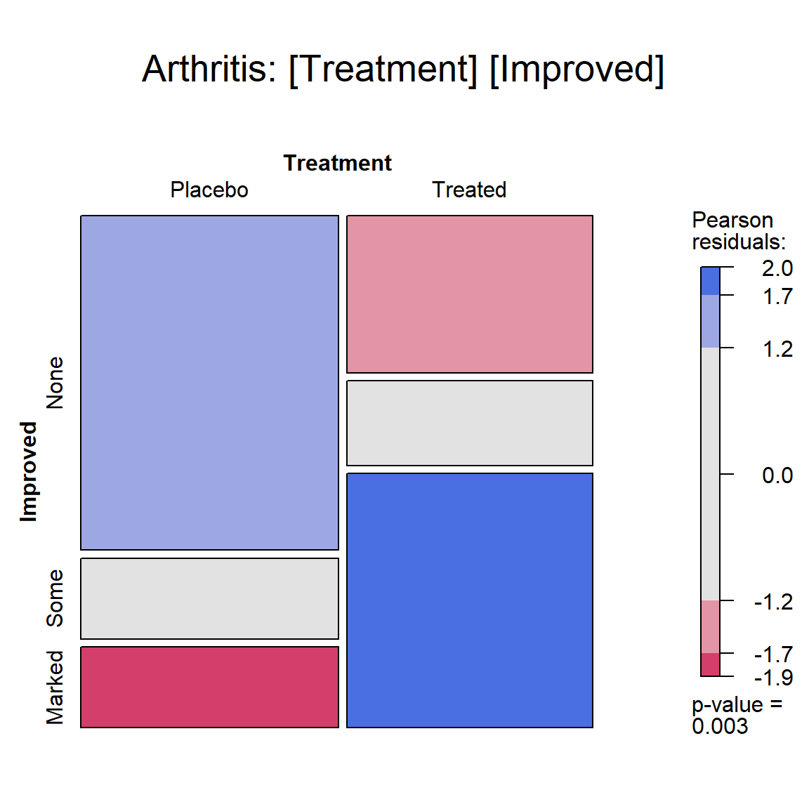
Mosaic plot for the Arthritis data, showing the marginal
model of independence for Treatment and Improved. Age, a covariate, and
Sex are ignored here.
Several data sets in the package illustrate the salutary effects of reordering factor levels in mosaic displays and other analyses. See:
The seriate package now contains a general method to permute the row and column variables in a table according to the result of a correspondence analysis, using scores on the first CA dimension.
Re-ordering dimensions
Finally, there are situations where, particularly for display
purposes, you want to re-order the dimensions of an \(n\)-way table, or change the labels for the
variables or levels. This is easy when the data are in table form:
aperm() permutes the dimensions, and assigning to
names and dimnames changes variable names and
level labels respectively. We will use the following version of
UCBAdmissions in @(sec:mantel) below. 1
UCB <- aperm(UCBAdmissions, c(2, 1, 3))
dimnames(UCB)[[2]] <- c("Yes", "No")
names(dimnames(UCB)) <- c("Sex", "Admit?", "Department")

# display as a flattened table
stats::ftable(UCB)
##               Department   A   B   C   D   E   F
## Sex    Admit?
## Male   Yes               512 353 120 138  53  22
##        No                313 207 205 279 138 351
## Female Yes                89  17 202 131  94  24
##        No                 19   8 391 244 299 317
structable()
For 3-way and larger tables the structable() function in
vcd provides a convenient and flexible tabular display. The
variables assigned to the rows and columns of a two-way display can be
specified by a model formula.
structable(HairEyeColor)                   # show the table: default
##              Eye Brown Hazel Green Blue
## Hair  Sex
## Black Male          32    10     3   11
##       Female        36     5     2    9
## Brown Male          53    25    15   50
##       Female        66    29    14   34
## Red   Male          10     7     7   10
##       Female        16     7     7    7
## Blond Male           3     5     8   30
##       Female         4     5     8   64

structable(Hair+Sex ~ Eye, HairEyeColor)   # specify col ~ row variables
##       Hair Black        Brown         Red        Blond
##       Sex   Male Female  Male Female Male Female  Male Female
## Eye
## Brown         32     36    53     66   10     16     3      4
## Hazel         10      5    25     29    7      7     5      5
## Green          3      2    15     14    7      7     8      8
## Blue          11      9    50     34   10      7    30     64
It also returns an object of class "structable" which
may be plotted with mosaic() (not shown here).
HSE < - structable(Hair+Sex ~ Eye, HairEyeColor)   # save structable object
mosaic(HSE)                                        # plot it
table() and friends
You can generate frequency tables from factor variables using the
table() function, tables of proportions using the
prop.table() function, and marginal frequencies using
margin.table().
For these examples, create some categorical vectors:
 n=500
 A <- factor(sample(c("a1","a2"), n, rep=TRUE))
 B <- factor(sample(c("b1","b2"), n, rep=TRUE))
 C <- factor(sample(c("c1","c2"), n, rep=TRUE))
 mydata <- data.frame(A,B,C)
These lines illustrate table-related functions:
# 2-Way Frequency Table
attach(mydata)
mytable <- table(A,B)   # A will be rows, B will be columns
mytable                 # print table
##     B
## A     b1  b2
##   a1 116 114
##   a2 138 132

margin.table(mytable, 1) # A frequencies (summed over B)
## A
##  a1  a2
## 230 270
margin.table(mytable, 2) # B frequencies (summed over A)
## B
##  b1  b2
## 254 246

prop.table(mytable)    # cell percentages
##     B
## A       b1    b2
##   a1 0.232 0.228
##   a2 0.276 0.264
prop.table(mytable, 1) # row percentages
##     B
## A           b1        b2
##   a1 0.5043478 0.4956522
##   a2 0.5111111 0.4888889
prop.table(mytable, 2) # column percentages
##     B
## A           b1        b2
##   a1 0.4566929 0.4634146
##   a2 0.5433071 0.5365854
table() can also generate multidimensional tables based
on 3 or more categorical variables. In this case, you can use the
ftable() or structable() function to print the
results more attractively.
# 3-Way Frequency Table
mytable <- table(A, B, C)
ftable(mytable)
##       C c1 c2
## A  B
## a1 b1   45 71
##    b2   59 55
## a2 b1   62 76
##    b2   76 56
table() ignores missing values by default. To include
NA as a category in counts, include the table option
exclude=NULL if the variable is a vector. If the variable
is a factor you have to create a new factor using .
xtabs()
The xtabs() function allows you to create
cross-tabulations of data using formula style input. This typically
works with case-form data supplied in a data frame or a matrix. The
result is a contingency table in array format, whose dimensions are
determined by the terms on the right side of the formula.
# 3-Way Frequency Table
mytable <- xtabs(~A+B+C, data=mydata)

ftable(mytable)    # print table
##       C c1 c2
## A  B
## a1 b1   45 71
##    b2   59 55
## a2 b1   62 76
##    b2   76 56

summary(mytable)   # chi-square test of indepedence
## Call: xtabs(formula = ~A + B + C, data = mydata)
## Number of cases in table: 500
## Number of factors: 3
## Test for independence of all factors:
##  Chisq = 9.888, df = 4, p-value = 0.04235
If a variable is included on the left side of the formula, it is assumed to be a vector of frequencies (useful if the data have already been tabulated in frequency form).
(GSStab <- xtabs(count ~ sex + party, data=GSS))
##         party
## sex      dem indep rep
##   female 279    73 225
##   male   165    47 191

summary(GSStab)
## Call: xtabs(formula = count ~ sex + party, data = GSS)
## Number of cases in table: 980
## Number of factors: 2
## Test for independence of all factors:
##  Chisq = 7.01, df = 2, p-value = 0.03005
Collapsing over table factors: aggregate(),
margin.table() and apply()
It sometimes happens that we have a data set with more variables or factors than we want to analyse, or else, having done some initial analyses, we decide that certain factors are not important, and so should be excluded from graphic displays by collapsing (summing) over them. For example, mosaic plots and fourfold displays are often simpler to construct from versions of the data collapsed over the factors which are not shown in the plots.
The appropriate tools to use again depend on the form in which the
data are represented— a case-form data frame, a frequency-form data
frame (aggregate()), or a table-form array or table object
(margin.table() or apply()).
When the data are in frequency form, and we want to produce another
frequency data frame, aggregate() is a handy tool, using
the argument FUN=sum to sum the frequency variable over the
factors not mentioned in the formula.
Example: The data frame
DaytonSurvey in the vcdExtra package
represents a \(2^5\) table giving the
frequencies of reported use (``ever used?’’) of alcohol, cigarettes and
marijuana in a sample of high school seniors, also classified by sex and
race.
data("DaytonSurvey", package="vcdExtra")
str(DaytonSurvey)
## 'data.frame':    32 obs. of  6 variables:
##  $ cigarette: Factor w/ 2 levels "Yes","No": 1 2 1 2 1 2 1 2 1 2 ...
##  $ alcohol  : Factor w/ 2 levels "Yes","No": 1 1 2 2 1 1 2 2 1 1 ...
##  $ marijuana: Factor w/ 2 levels "Yes","No": 1 1 1 1 2 2 2 2 1 1 ...
##  $ sex      : Factor w/ 2 levels "female","male": 1 1 1 1 1 1 1 1 2 2 ...
##  $ race     : Factor w/ 2 levels "white","other": 1 1 1 1 1 1 1 1 1 1 ...
##  $ Freq     : num  405 13 1 1 268 218 17 117 453 28 ...
head(DaytonSurvey)
##   cigarette alcohol marijuana    sex  race Freq
## 1       Yes     Yes       Yes female white  405
## 2        No     Yes       Yes female white   13
## 3       Yes      No       Yes female white    1
## 4        No      No       Yes female white    1
## 5       Yes     Yes        No female white  268
## 6        No     Yes        No female white  218
To focus on the associations among the substances, we want to
collapse over sex and race. The right-hand side of the formula used in
the call to aggregate() gives the factors to be retained in
the new frequency data frame, Dayton.ACM.df.
# data in frequency form
# collapse over sex and race
Dayton.ACM.df <- aggregate(Freq ~ cigarette+alcohol+marijuana,
                           data=DaytonSurvey,
                           FUN=sum)
Dayton.ACM.df
##   cigarette alcohol marijuana Freq
## 1       Yes     Yes       Yes  911
## 2        No     Yes       Yes   44
## 3       Yes      No       Yes    3
## 4        No      No       Yes    2
## 5       Yes     Yes        No  538
## 6        No     Yes        No  456
## 7       Yes      No        No   43
## 8        No      No        No  279
When the data are in table form, and we want to produce another
table, apply() with FUN=sum can be used in a
similar way to sum the table over dimensions not mentioned in the
MARGIN argument. margin.table() is just a
wrapper for apply() using the sum()
function.
Example: To illustrate, we first convert
the DaytonSurvey to a 5-way table using
xtabs(), giving Dayton.tab.
# in table form
Dayton.tab <- xtabs(Freq ~ cigarette+alcohol+marijuana+sex+race,
                    data=DaytonSurvey)
structable(cigarette+alcohol+marijuana ~ sex+race,
           data=Dayton.tab)
##              cigarette Yes              No
##              alcohol   Yes      No     Yes      No
##              marijuana Yes  No Yes  No Yes  No Yes  No
## sex    race
## female white           405 268   1  17  13 218   1 117
##        other            23  23   0   1   2  19   0  12
## male   white           453 228   1  17  28 201   1 133
##        other            30  19   1   8   1  18   0  17
Then, use apply() on Dayton.tab to give the
3-way table Dayton.ACM.tab summed over sex and race. The
elements in this new table are the column sums for
Dayton.tab shown by structable() just
above.
# collapse over sex and race
Dayton.ACM.tab <- apply(Dayton.tab, MARGIN=1:3, FUN=sum)
Dayton.ACM.tab <- margin.table(Dayton.tab, 1:3)   # same result

structable(cigarette+alcohol ~ marijuana, data=Dayton.ACM.tab)
##           cigarette Yes      No
##           alcohol   Yes  No Yes  No
## marijuana
## Yes                 911   3  44   2
## No                  538  43 456 279
Many of these operations can be performed using the
**ply() functions in the plyr
package. For example, with the data in a frequency form data frame, use
ddply() to collapse over unmentioned factors, and
plyr::summarise() as the function to be applied to each
piece.
library(plyr)
Dayton.ACM.df <- plyr::ddply(DaytonSurvey,
                             .(cigarette, alcohol, marijuana),
                             plyr::summarise, Freq=sum(Freq))

Dayton.ACM.df
##   cigarette alcohol marijuana Freq
## 1       Yes     Yes       Yes  911
## 2       Yes     Yes        No  538
## 3       Yes      No       Yes    3
## 4       Yes      No        No   43
## 5        No     Yes       Yes   44
## 6        No     Yes        No  456
## 7        No      No       Yes    2
## 8        No      No        No  279
Collapsing table levels: collapse.table()
A related problem arises when we have a table or array and for some
purpose we want to reduce the number of levels of some factors by
summing subsets of the frequencies. For example, we may have initially
coded Age in 10-year intervals, and decide that, either for analysis or
display purposes, we want to reduce Age to 20-year intervals. The
collapse.table() function in vcdExtra was
designed for this purpose.
Example: Create a 3-way table, and collapse Age from 10-year to 20-year intervals. First, we generate a \(2 \times 6 \times 3\) table of random counts from a Poisson distribution with mean of 100.
# create some sample data in frequency form
sex <- c("Male", "Female")
age <- c("10-19", "20-29",  "30-39", "40-49", "50-59", "60-69")
education <- c("low", 'med', 'high')
data <- expand.grid(sex=sex, age=age, education=education)
counts <- rpois(36, 100)   # random Possion cell frequencies
data <- cbind(data, counts)

# make it into a 3-way table
t1 <- xtabs(counts ~ sex + age + education, data=data)
structable(t1)
##                  age 10-19 20-29 30-39 40-49 50-59 60-69
## sex    education
## Male   low              98   105   104    90    90   101
##        med              97   105   101    88    97   107
##        high             99   101   109    88    99    96
## Female low             102   117   101   105    85    88
##        med             106    84    92   116   110    96
##        high            106    96   121    91   107   102
Now collapse age to 20-year intervals, and
education to 2 levels. In the arguments, levels of
age and education given the same label are
summed in the resulting smaller table.
# collapse age to 3 levels, education to 2 levels
t2 <- collapse.table(t1,
         age=c("10-29", "10-29",  "30-49", "30-49", "50-69", "50-69"),
         education=c("<high", "<high", "high"))
structable(t2)
##                  age 10-29 30-49 50-69
## sex    education
## Male   <high           405   383   395
##        high            200   197   195
## Female <high           409   414   379
##        high            202   212   209
Collapsing table levels: dplyr
For data sets in frequency form or case form, factor levels can be
collapsed by recoding the levels to some grouping. One handy function
for this is dplyr::case_match()
Example:
The vcdExtra::Titanicp data set contains information on
1309 passengers on the RMS Titanic, including
sibsp, the number of (0:8) siblings or spouses aboard, and
parch (0:6), the number of parents or children aboard, but
the table is quite sparse.
table(Titanicp$sibsp, Titanicp$parch)
##
##       0   1   2   3   4   5   6   9
##   0 790  52  43   2   2   2   0   0
##   1 183  90  29   5   4   4   2   2
##   2  26   9   6   1   0   0   0   0
##   3   3   9   8   0   0   0   0   0
##   4   0  10  12   0   0   0   0   0
##   5   0   0   6   0   0   0   0   0
##   8   0   0   9   0   0   0   0   0
For purposes of analysis, we might want to collapse both of these to
the levels 0, 1, 2+. Here’s how:
library(dplyr)
Titanicp <- Titanicp |>
  mutate(sibspF = case_match(sibsp,
                            0 ~ "0",
                            1 ~ "1",
                            2:max(sibsp) ~ "2+")) |>
  mutate(sibspF = ordered(sibspF)) |>
  mutate(parchF = case_match(parch,
                             0 ~ "0",
                             1 ~ "1",
                             2:max(parch) ~ "2+")) |>
  mutate(parchF = ordered(parchF))

table(Titanicp$sibspF, Titanicp$parchF)
##
##        0   1  2+
##   0  790  52  49
##   1  183  90  46
##   2+  29  28  42
car::recode() is a similar function, but with a less
convenient interface.
The forcats
package provides a collection of functions for reordering the levels of
a factor or grouping categories acording to their frequency:
-
forcats::fct_reorder(): Reorder a factor by another variable. -
forcats::fct_infreq(): Reorder a factor by the frequency of values. -
forcats::fct_relevel(): Change the order of a factor by hand. -
forcats::fct_lump(): Collapse the least/most frequent values of a factor into “other”. -
forcats::fct_collapse(): Collapse factor levels into manually defined groups. -
forcats::fct_recode(): Change factor levels by hand.
Converting among frequency tables and data frames
As we’ve seen, a given contingency table can be represented equivalently in different forms, but some R functions were designed for one particular representation.
The table below shows some handy tools for converting from one form to another.
| From this | To this | ||
|---|---|---|---|
| Case form | Frequency form | Table form | |
| Case form | noop | xtabs(~A+B) |
table(A,B) |
| Frequency form | expand.dft(X) |
noop | xtabs(count~A+B) |
| Table form | expand.dft(X) |
as.data.frame(X) |
noop |
For example, a contingency table in table form (an object of
class(table)) can be converted to a data.frame with
as.data.frame(). 2 The resulting data.frame
contains columns representing the classifying factors and the table
entries (as a column named by the responseName argument,
defaulting to Freq. This is the inverse of
xtabs().
Example: Convert the GSStab in
table form to a data.frame in frequency form.
as.data.frame(GSStab)
##      sex party Freq
## 1 female   dem  279
## 2   male   dem  165
## 3 female indep   73
## 4   male indep   47
## 5 female   rep  225
## 6 male rep 191Example: Convert the Arthritis
data in case form to a 3-way table of Treatment \(\times\) Sex \(\times\) Improved. Note the
use of with() to avoid having to use
Arthritis\$Treatment etc. within the call to
table().% 3
Art.tab <- with(Arthritis, table(Treatment, Sex, Improved))
str(Art.tab)
##  'table' int [1:2, 1:2, 1:3] 19 6 10 7 7 5 0 2 6 16 ...
##  - attr(*, "dimnames")=List of 3
##   ..$ Treatment: chr [1:2] "Placebo" "Treated"
##   ..$ Sex      : chr [1:2] "Female" "Male"
##   ..$ Improved : chr [1:3] "None" "Some" "Marked"

ftable(Art.tab)
##                  Improved None Some Marked
## Treatment Sex
## Placebo   Female            19    7      6
##           Male              10    0      1
## Treated   Female             6    5     16
##           Male               7    2      5
There may also be times that you will need an equivalent case form
data.frame with factors representing the table variables
rather than the frequency table. For example, the mca()
function in package MASS only operates on data in this
format. Marc Schwartz initially provided code for
expand.dft() on the Rhelp mailing list for converting a
table back into a case form data.frame. This function is
included in vcdExtra.
Example: Convert the Arthritis
data in table form (Art.tab) back to a
data.frame in case form, with factors
Treatment, Sex and Improved.
Art.df <- expand.dft(Art.tab)
str(Art.df)
## 'data.frame':    84 obs. of  3 variables:
##  $ Treatment: chr  "Placebo" "Placebo" "Placebo" "Placebo" ...
##  $ Sex      : chr  "Female" "Female" "Female" "Female" ...
##  $ Improved : chr  "None" "None" "None" "None" ...
A complex example
If you’ve followed so far, you’re ready for a more complicated
example. The data file, tv.dat represents a 4-way table of
size \(5 \times 11 \times 5 \times 3\)
where the table variables (unnamed in the file) are read as
V1 – V4, and the cell frequency is read as
V5. The file, stored in the doc/extdata
directory of vcdExtra, can be read as follows:
tv.data<-read.table(system.file("extdata","tv.dat", package="vcdExtra"))
head(tv.data,5)
##   V1 V2 V3 V4 V5
## 1  1  1  1  1  6
## 2  2  1  1  1 18
## 3  3  1  1  1  6
## 4  4  1  1  1  2
## 5  5  1  1  1 11
For a local file, just use read.table() in this
form:
tv.data<-read.table("C:/R/data/tv.dat")The data tv.dat came from the initial implementation of
mosaic displays in R by Jay Emerson. In turn, they came from the initial
development of mosaic displays (Hartigan &
Kleiner, 1984) that illustrated the method with data on a large
sample of TV viewers whose behavior had been recorded for the Neilsen
ratings. This data set contains sample television audience data from
Neilsen Media Research for the week starting November 6, 1995.
The table variables are:
-
V1– values 1:5 correspond to the days Monday–Friday; -
V2– values 1:11 correspond to the quarter hour times 8:00PM through 10:30PM; -
V3– values 1:5 correspond to ABC, CBS, NBC, Fox, and non-network choices; -
V4– values 1:3 correspond to transition states: turn the television Off, Switch channels, or Persist in viewing the current channel.
We are interested just the cell frequencies, and rely on the facts that the
- the table is complete— there are no missing cells, so
nrow(tv.data)= 825; - the observations are ordered so that
V1varies most rapidly andV4most slowly. From this, we can just extract the frequency column and reshape it into an array. [That would be dangerous if any observations were out of order.]
TV <- array(tv.data[,5], dim=c(5,11,5,3))
dimnames(TV) <- list(c("Monday","Tuesday","Wednesday","Thursday","Friday"),
                     c("8:00","8:15","8:30","8:45","9:00","9:15","9:30",
                       "9:45","10:00","10:15","10:30"),
                     c("ABC","CBS","NBC","Fox","Other"),
                     c("Off","Switch","Persist"))

names(dimnames(TV))<-c("Day", "Time", "Network", "State")
More generally (even if there are missing cells), we can use
xtabs() (or plyr::daply()) to do the
cross-tabulation, using V5 as the frequency variable.
Here’s how to do this same operation with xtabs():
TV <- xtabs(V5 ~ ., data=tv.data)
dimnames(TV) <- list(Day = c("Monday","Tuesday","Wednesday","Thursday","Friday"),
                     Time = c("8:00","8:15","8:30","8:45","9:00","9:15","9:30",
                              "9:45","10:00","10:15","10:30"),
                     Network = c("ABC","CBS","NBC","Fox","Other"),
                     State = c("Off","Switch","Persist"))

# table dimensions
dim(TV)
But this 4-way table is too large and awkward to work with. Among the networks, Fox and Other occur infrequently. We can also cut it down to a 3-way table by considering only viewers who persist with the current station. 4
TV2 <- TV[,,1:3,]      # keep only ABC, CBS, NBC
TV2 <- TV2[,,,3]       # keep only Persist -- now a 3 way table
structable(TV2)
##                   Time 8:00 8:15 8:30 8:45 9:00 9:15 9:30 9:45 10:00 10:15 10:30
## Day       Network
## Monday    ABC           146  151  156   83  325  350  386  340   352   280   278
##           CBS           337  293  304  233  311  251  241  164   252   265   272
##           NBC           263  219  236  140  226  235  239  246   279   263   283
## Tuesday   ABC           244  181  231  205  385  283  345  192   329   351   364
##           CBS           173  180  184  109  218  235  256  250   274   263   261
##           NBC           315  254  280  241  370  214  195  111   188   190   210
## Wednesday ABC           233  161  194  156  339  264  279  140   237   228   203
##           CBS           158  126  207   59   98  103  122   86   109   105   110
##           NBC           134  146  166   66  194  230  264  143   274   289   306
## Thursday  ABC           174  183  197  181  187  198  211   86   110   122   117
##           CBS           196  185  195  104  106  116  116   47   102    84    84
##           NBC           515  463  472  477  590  473  446  349   649   705   747
## Friday    ABC           294  281  305  239  278  246  245  138   246   232   233
##           CBS           130  144  154   81  129  153  136  126   138   136   152
##           NBC           195  220  248  160  172  164  169   85   183   198   204
Finally, for some purposes, we might want to collapse the 11 times
into a smaller number. Half-hour time slots make more sense. Here, we
use as.data.frame.table() to convert the table back to a
data frame, levels() to re-assign the values of
Time, and finally, xtabs() to give a new,
collapsed frequency table.
TV.df <- as.data.frame.table(TV2)
levels(TV.df$Time) <- c(rep("8:00", 2),
                        rep("8:30", 2),
                        rep("9:00", 2),
                        rep("9:30", 2),
                        rep("10:00",2),
                            "10:30"
                        )

TV3 <- xtabs(Freq ~ Day + Time + Network, TV.df)

structable(Day ~ Time+Network, TV3)
##               Day Monday Tuesday Wednesday Thursday Friday
## Time  Network
## 8:00  ABC            297     425       394      357    575
##       CBS            630     353       284      381    274
##       NBC            482     569       280      978    415
## 8:30  ABC            239     436       350      378    544
##       CBS            537     293       266      299    235
##       NBC            376     521       232      949    408
## 9:00  ABC            675     668       603      385    524
##       CBS            562     453       201      222    282
##       NBC            461     584       424     1063    336
## 9:30  ABC            726     537       419      297    383
##       CBS            405     506       208      163    262
##       NBC            485     306       407      795    254
## 10:00 ABC            632     680       465      232    478
##       CBS            517     537       214      186    274
##       NBC            542     378       563     1354    381
## 10:30 ABC            278     364       203      117    233
##       CBS            272     261       110       84    152
##       NBC            283     210       306      747    204
We’ve come this far, so we might as well show a mosaic display. This is analogous to that used by Hartigan & Kleiner (1984).
mosaic(TV3, shade = TRUE,
       labeling = labeling_border(rot_labels = c(0, 0, 0, 90)))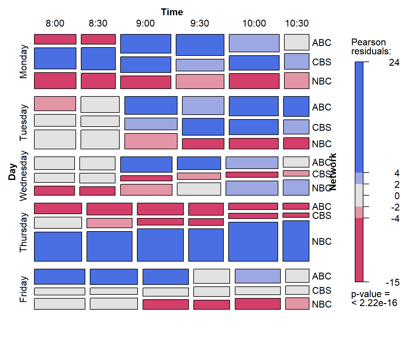
This mosaic displays can be read at several levels, corresponding to the successive splits of the tiles and the residual shading. Several trends are clear for viewers who persist:
- Overall, there are about the same number of viewers on each weekday, with slightly more on Thursday.
- Looking at time slots, viewership is slightly greater from 9:00 - 10:00 overall and also 8:00 - 9:00 on Thursday and Friday
From the residual shading of the tiles:
- Monday: CBS dominates in all time slots.
- Tuesday” ABC and CBS dominate after 9:00
- Thursday: is a largely NBC day
- Friday: ABC dominates in the early evening