To make the preliminary test on variances is rather like putting to sea in a rowing boat to find out whether conditions are sufficiently calm for an ocean liner to leave port. — G. E. P. Box (1953)
This chapter concerns the extension of tests of homogeneity of variance from the classical univariate ANOVA setting to the analogous multivariate (MANOVA) setting. Such tests are a routine but important aspect of data analysis, as particular violations can drastically impact model estimates (Lix & Keselman, 1996).
We provide some answers to the following questions:
Visualization: How can we visualize differences among group variances and covariance matrices, perhaps in a way that is analogous to what is done to visualize differences among group means? As will be illustrated, differences among covariance matrices can be comprised of spread in overall size (“scatter”) and shape (“orientation”). These can be seen in data space with data ellipses, particularly if the data is centered by shifting all groups to the grand mean,
Low-D views: When there are more than a few response variables, what low-dimensional views can show the most interesting properties related to the equality of covariance matrices? Projecting the data into the space of the principal components serves well again here. Surprisingly, we will see that the small dimensions contain useful information about differences among the group covariance matrices.
Other statistics: Box’s \(M\)-test is most widely used. Are there other worthwhile test statistics? We will see that graphics methods suggest alternatives.
The following subsections provide a capsule summary of the issues in this topic. Most of the discussion is couched in terms of a one-way design for simplicity, but the same ideas can apply to two-way (and higher) designs, where a “group” factor is defined as the product combination (interaction) of two or more factor variables. When there are also numeric covariates, this topic can also be extended to the multivariate analysis of covaraiance (MANCOVA) setting. This can be accomplished by applying these techniques to the residuals from predictions by the covariates alone.
Packages
In this chapter we use the following packages. Load them now
13.1 Homogeneity of Variance in Univariate ANOVA
In classical (Gaussian) univariate ANOVA models, the main interest is typically on tests of mean differences in a response \(y\) according to one or more factors. The validity of the typical \(F\) test, however, relies on the assumption of homogeneity of variance: all groups have the same (or similar) variance, \[ \sigma_1^2 = \sigma_2^2 = \cdots = \sigma_g^2 \; . \]
It turns out that the \(F\) test for differences in means is relatively robust to violation of this assumption (Harwell et al., 1992), as long as the group sizes are roughly equal.1
A variety of classical test statistics for homogeneity of variance are available, including Hartley’s \(F_{max}\) (Hartley, 1950), Cochran’s C (Cochran, 1941),and Bartlett’s test (Bartlett, 1937), but these have been found to have terrible statistical properties (Rogan & Keselman, 1977), which prompted Box’s famous quote.
Levene (1960) introduced a different form of test, based on the simple idea that when variances are equal across groups, the average absolute values of differences between the observations and group means will also be equal, i.e., substituting an \(L_1\) norm for the \(L_2\) norm of variance. In a one-way design, this is equivalent to a test of group differences in the means of the auxilliary variable \(z_{ij} = | y_{ij} - \bar{y}_i |\).
More robust versions of this test were proposed by Brown & Forsythe (1974). These tests substitute the group mean by either the group median or a trimmed mean in the ANOVA of the absolute deviations, and should be almost always preferred to Levene’s version. See Conover et al. (1981) for an early review and Gastwirth et al. (2009) for a general discussion of these tests. In what follows, we refer to this class of tests as “Levene-type” tests and suggest a multivariate extension described below (Section 13.2).
13.2 Homogeneity of variance in ANOVA
13.3 Homogeneity of variance in MANOVA
In the MANOVA context, the main emphasis, of course, is on differences among mean vectors, testing \[ H_0 : \mathbf{\mu}_1 = \mathbf{\mu}_2 = \cdots = \mathbf{\mu}_g \; . \] However, the standard test statistics (Wilks’ Lambda, Hotelling-Lawley trace, Pillai-Bartlett trace, Roy’s maximum root) rely upon the analogous assumption that the within-group covariance matrices for all groups are equal, \[ \mathbf{\Sigma}_1 = \mathbf{\Sigma}_2 = \cdots = \mathbf{\Sigma}_g \; . \]
Insert pairs covEllipses for penguins data
To preview the main example, Figure 13.1 shows data ellipses for the main size variables in the palmerpenguins::penguins data.
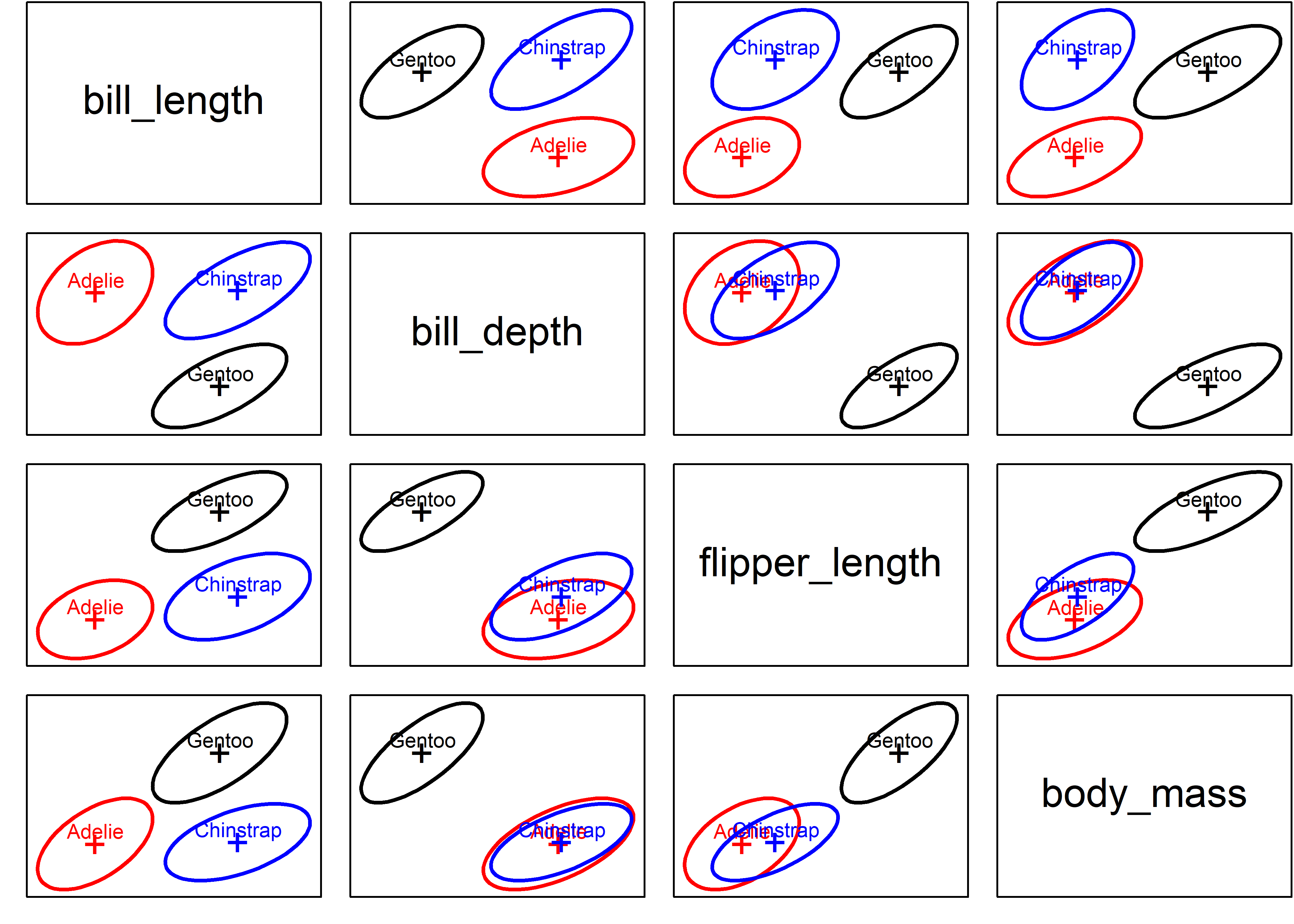
They covariance ellipses look pretty similar in size, shape and orientation. But what does Box’s M test (described below) say? As you can see, it concludes strongly against the null hypothesis.
13.4 Assessing heterogeneity of covariance matrices: Box’s M test
Box (1949) proposed the following likelihood-ratio test (LRT) statistic for testing the hypothesis of equal covariance matrices, \[ M = (N -g) \ln \;|\; \mathbf{S}_p \;|\; - \sum_{i=1}^g (n_i -1) \ln \;|\; \mathbf{S}_i \;|\; \; , \] {eq-boxm}
where \(N = \sum n_i\) is the total sample size and \(\mathbf{S}_p = (N-g)^{-1} \sum_{i=1}^g (n_i - 1) \mathbf{S}_i\) is the pooled covariance matrix. \(M\) can thus be thought of as a ratio of the determinant of the pooled \(\mathbf{S}_p\) to the geometric mean of the determinants of the separate \(\mathbf{S}_i\).
In practice, there are various transformations of the value of \(M\) to yield a test statistic with an approximately known distribution (Timm, 1975). Roughly speaking, when each \(n_i > 20\), a \(\chi^2\) approximation is often used; otherwise an \(F\) approximation is known to be more accurate.
Asymptotically, \(-2 \ln (M)\) has a \(\chi^2\) distribution. The \(\chi^2\) approximation due to Box (1949, 1950) is that \[ X^2 = -2 (1-c_1) \ln (M) \quad \sim \quad \chi^2_{df} \] with \(df = (g-1) p (p+1)/2\) degrees of freedom, and a bias correction constant: \[ c_1 = \left( \sum_i \frac{1}{n_i -1} - \frac{1}{N-g} \right) \frac{2p^2 +3p -1}{6 (p+1)(g-1)} \; . \]
In this form, Bartlett’s test for equality of variances in the univariate case is the special case of Box’s M when there is only one response variable, so Bartlett’s test is sometimes used as univariate follow-up to determine which response variables show heterogeneity of variance.
Yet, like its univariate counterpart, Box’s test is well-known to be highly sensitive to violation of (multivariate) normality and the presence of outliers. For example, Tiku & Balakrishnan (1984) concluded from simulation studies that the normal-theory LRT provides poor control of Type I error under even modest departures from normality. O’Brien (1992) proposed some robust alternatives, and showed that Box’s normal theory approximation suffered both in controlling the null size of the test and in power. Zhang & Boos (1992) also carried out simulation studies with similar conclusions and used bootstrap methods to obtain corrected critical values.
13.5 Visualizing heterogeneity
The goal of this chapter is to use the above background as a platform for discussing approaches to visualizing and testing the heterogeneity of covariance matrices in multivariate designs. While researchers often rely on a single number to determine if their data have met a particular threshold, such compression will often obscure interesting information, particularly when a test concludes that differences exist, and one is left to wonder ``why?’’. It is within this context where, again, visualizations often reign supreme. In fact, we find it somewhat surprising that this issue has not been addressed before graphically in any systematic way. TODO: cut this down
In what follows, we propose three visualization-based approaches to questions of heterogeneity of covariance in MANOVA designs:
direct visualization of the information in the \(\mathbf{S}_i\) and \(\mathbf{S}_p\) using data ellipsoids to show size and shape as minimal schematic summaries;
a simple dotplot of the components of Box’s M test: the log determinants of the \(\mathbf{S}_i\) together with that of the pooled \(\mathbf{S}_p\). Extensions of these simple plots raise the question of whether measures of heterogeneity other than that captured in Box’s test might also be useful; and,
the connection between Levene-type tests and an ANOVA (of centered absolute differences) suggests a parallel with a multivariate extension of Levene-type tests and a MANOVA. We explore this with a version of Hypothesis-Error (HE) plots we have found useful for visualizing mean differences in MANOVA designs.
#> Writing packages to  C:/R/Projects/Vis-MLM-book/bib/pkgs.txt
#> 9  packages used here:
#> broom, candisc, car, carData, dplyr, ggplot2, heplots, knitr, tidyrIf group sizes are greatly unequal and homogeneity of variance is violated, then the \(F\) statistic is too liberal (\(p\) values too large) when large sample variances are associated with small group sizes. Conversely, the \(F\) statistic is too conservative if large variances are associated with large group sizes.↩︎