This chapter may be moved from the printed PDF copy to an online Appendix.
For ease of exposition, the chapters in Part IV of this book used small examples to illustrate the statistical and visualization aspects of the techniques as they were described. Some of the main examples were spread over Chapters 10–13 to illustrate the specific statistical and graphical methods of those chapters.
Here I present more complete analyses of a few datasets to place the methods of this book in the wider research context. I illustrate a sequence of steps, starting with research questions involved and proceeding to the graphical, computing and statistical methods of this book required to understand and explain these data.1
Packages
In this chapter I use the following packages. Load them now.
14.1 Neuro- and Social-cognitive measures in psychiatric groups
A Ph.D. dissertation by Laura Hartman (2016) at York University was designed as a test case of ideas about whether cognitive aspects of clinical patients could be useful in understanding schizophrenia (Heinrichs et al., 2015). Her studies attempted to evaluate whether and how clinical patients diagnosed (on the DSM-IV) as schizophrenic or with a schizoaffective disorder could be distinguished from each other and from a normal, control sample on collections of standardized tests in the following domains:
Neuro-cognitive: processing speed, attention, verbal learning, visual learning and problem solving;
Social-cognitive: managing emotions, theory of mind, externalizing, personalizing bias.
The study is an important contribution to clinical research because the two diagnostic categories are subtly different and their manifest symptoms often overlap. Yet clinically, they’re very different and often require different treatments. A key difference between schizoaffective disorder and schizophrenia is the prominence of mood disorder involving bipolar, manic and depressive moods. With schizoaffective disorder, mood disorders are front and center. With schizophrenia, that is not a dominant part of the disorder, but psychotic ideation (hearing voices, seeing imaginary people) is.
14.1.1 Research questions
This example is concerned with the following substantitive questions:
To what extent can patients diagnosed as schizophrenic or with schizoaffective disorder be distinguished from each other and from a normal control sample using a well-validated, comprehensive neurocognitive battery specifically designed for individuals with psychosis (Heinrichs et al., 2015)?
If the groups differ, do any of the cognitive domains show particularly larger or smaller differences among these groups?
Do the neurocognitive measures discriminate among the in the same or different ways? If different, how many separate aspects or dimensions are distinguished?
Apart from the research interest, it could aid diagnosis and treatment if these similar mental disorders could be distinguished by tests in the cognitive domain.
14.1.2 Data
The clinical sample comprised 116 male and female patients who met the following criteria: 1) a diagnosis of schizophrenia (\(n\) = 70) or schizoaffective disorder (\(n\) = 46) confirmed by the Structured Clinical Interview for DSM-IV-TR Axis I Disorders; 2) were outpatients; 3) a history free of developmental or learning disability; 4) age 18-65; 5) a history free of neurological or endocrine disorder; and 6) no concurrent diagnosis of substance use disorder. Non-psychiatric control participants (\(n\) = 146) were screened for medical and psychiatric illness and history of substance abuse and were recruited from three outpatient clinics. The dataset is heplots::NeuroCog.
data(NeuroCog, package="heplots")
str(NeuroCog)
# 'data.frame': 242 obs. of  10 variables:
#  $ Dx       : Factor w/ 3 levels "Schizophrenia",..: 1 1 1 1 1 1 1 1 1 1 ...
#   ..- attr(*, "contrasts")= num [1:3, 1:2] -0.5 -0.5 1 1 -1 0
#   .. ..- attr(*, "dimnames")=List of 2
#   .. .. ..$ : chr [1:3] "Schizophrenia" "Schizoaffective" "Control"
#   .. .. ..$ : NULL
#  $ Speed    : int  19 8 14 7 21 31 -1 17 7 37 ...
#  $ Attention: int  9 25 23 18 9 10 8 20 30 15 ...
#  $ Memory   : int  19 15 15 14 35 26 3 27 26 17 ...
#  $ Verbal   : int  33 28 20 34 28 29 20 30 26 33 ...
#  $ Visual   : int  24 24 13 16 29 21 12 32 27 21 ...
#  $ ProbSolv : int  39 40 32 31 45 33 29 29 30 33 ...
#  $ SocialCog: int  28 37 24 36 28 28 28 44 39 24 ...
#  $ Age      : int  44 26 55 53 51 21 53 56 48 46 ...
#  $ Sex      : Factor w/ 2 levels "Female","Male": 1 2 1 2 2 2 2 1 2 1 ...
#  - attr(*, "na.action")= 'omit' Named int [1:21] 1 2 3 4 5 6 7 8 9 10 ...
#   ..- attr(*, "names")= chr [1:21] "1" "2" "3" "4" ...
The diagnostic classification variable is called Dx in the dataset. To facilitate answering questions regarding group differences, the following contrasts were applied: the first column compares the control group to the average of the diagnosed groups, the second compares the schizophrenia group against the schizoaffective group.
contrasts(NeuroCog$Dx)
#                 [,1] [,2]
# Schizophrenia   -0.5    1
# Schizoaffective -0.5   -1
# Control          1.0    0
In this analysis, I ignore the SocialCog variable because aspects of social cognition were measured more extensively in a separate dataset discussed below (sec-social-cog). The primary focus here is on the the cognitive and perceptual variables Attention : ProbSolv.
14.1.3 A first look
As always, plot the data first! We want an overview of the distributions of the variables to see the centers, spread, shape and possible outliers for each group on each variable.
The plot below combines the use of boxplots and violin plots to give an informative display. As we saw earlier (e.g., sec-NLSY-mmra), doing this with ggplot2 requires reshaping the data to long format.
# Reshape from wide to long
NC_long <- NeuroCog |>
  dplyr::select(-SocialCog, -Age, -Sex) |>
  tidyr::gather(key = response, value = "value", Speed:ProbSolv)
# view 3 observations per group and measure
NC_long |>
  group_by(Dx) |>
  sample_n(3) |> ungroup()
# # A tibble: 9 × 3
#   Dx              response  value
#   <fct>           <chr>     <int>
# 1 Schizophrenia   Speed        39
# 2 Schizophrenia   Visual       21
# 3 Schizophrenia   Memory       40
# 4 Schizoaffective ProbSolv     40
# 5 Schizoaffective Speed        25
# 6 Schizoaffective Verbal       48
# 7 Control         Speed        33
# 8 Control         ProbSolv     43
# 9 Control         Attention    37
In the plot, we take care to adjust the transparency (alpha) values for the points, violin plots and boxplots so that all can be seen. Options for geom_boxplot() are used to give these greater visual prominence.
Code
ggplot(NC_long, aes(x=Dx, y=value, fill=Dx)) +
  geom_jitter(shape=16, alpha=0.8, size=1, width=0.2) +
  geom_violin(alpha = 0.1) +
  geom_boxplot(width=0.5, alpha=0.4,
               outlier.alpha=1,
               outlier.size = 3, outlier.color = "red") +
  scale_x_discrete(labels = c("Schizo", "SchizAff", "Control")) +
  facet_wrap(~response, scales = "free_y", as.table = FALSE) +
  theme_bw() +
  theme(legend.position="bottom",
        axis.title = element_text(size = rel(1.2)),
        axis.text  = element_text(face = "bold"),
        strip.text = element_text(size = rel(1.2)))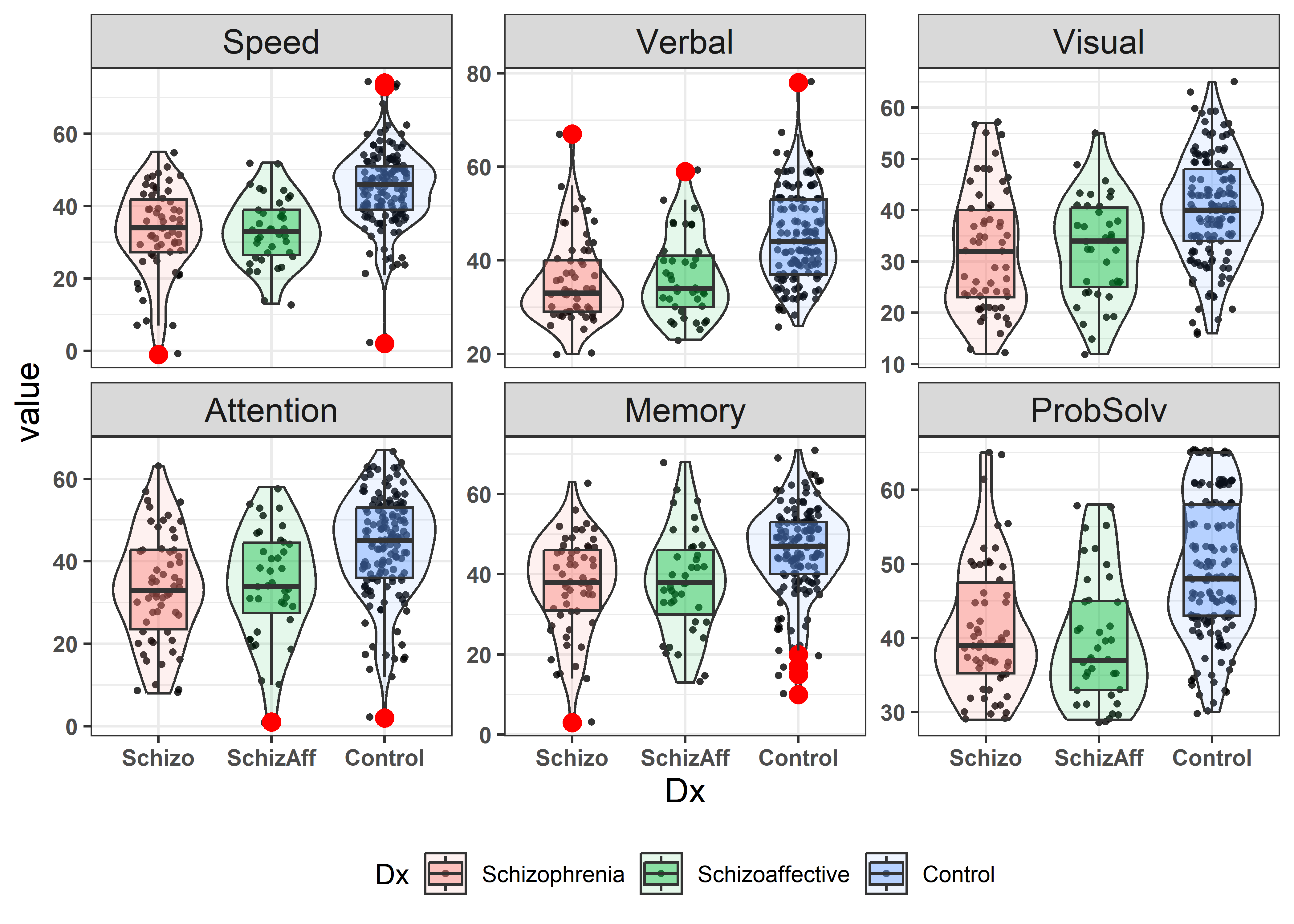
NeuroCog data.
We can see that the control participants score higher on all measures, but there is no consistent pattern of medians for the two patient groups. But these univariate summaries do not inform about the relations among variables.
14.2 Bivariate views
Corrgram
With this many variables, it is useful to view the correlations among them in a corrgram (sec-corrgram), giving a high-level reconnaissance. As noted earlier, the corrgram::corrgram() function can enhance perception by permuting the variables in the order of their variable vectors in a biplot, so more highly correlated variables are adjacent in the plot, an example of effect ordering for data displays (Friendly & Kwan, 2003).
NeuroCog |>
  select(-Dx, -SocialCog) |>
  corrgram(order = TRUE,
           diag.panel = panel.density,
           upper.panel = panel.pie)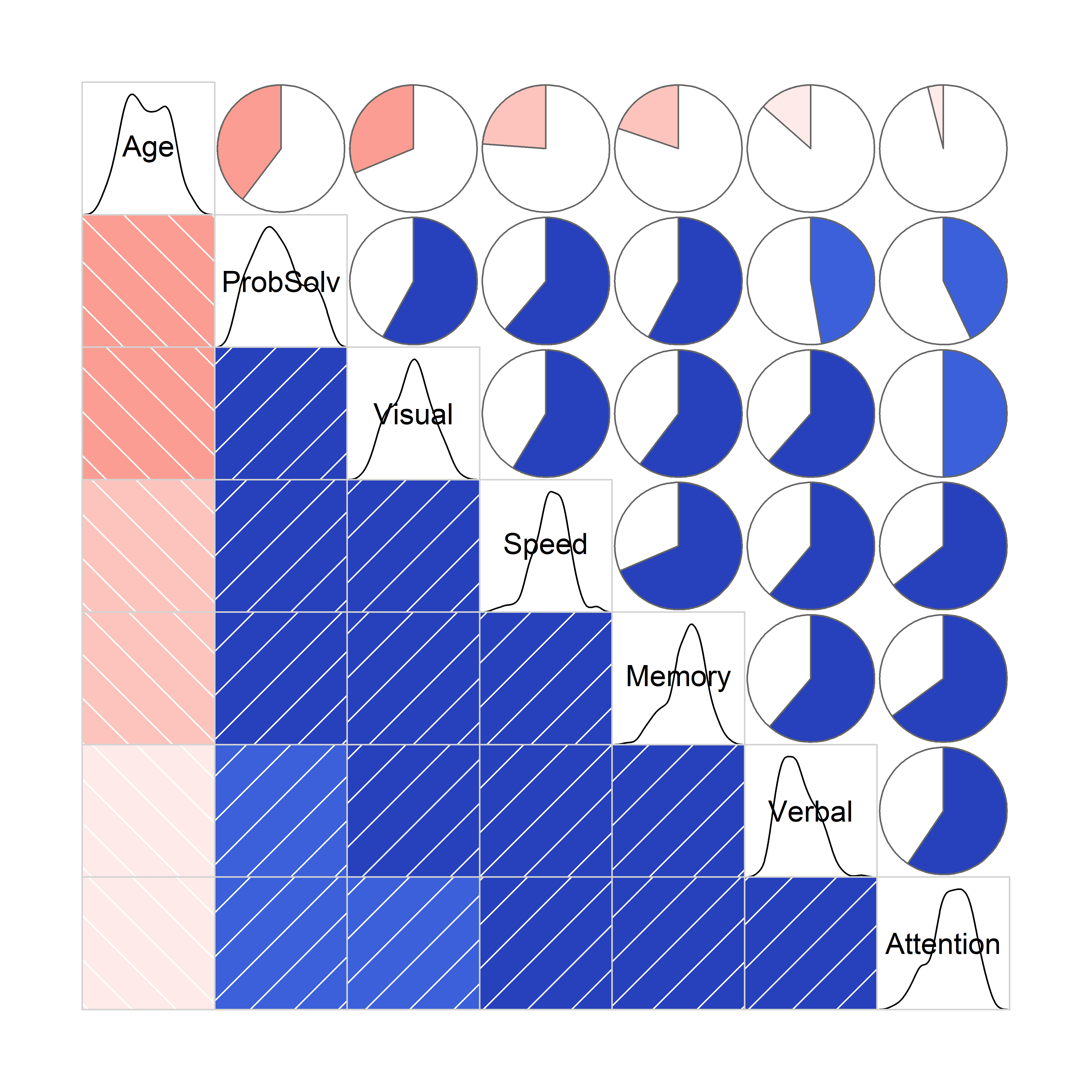
NeuroCog data. The upper and lower triangles use two different ways of encoding the value of the correlation for each pair of variables.
In this plot you can see that adjacent variables are more highly correlated than those more widely separated. The diagonal panels show that most variables are reasonably symmetric in their distributions. Age, not included in this analysis is negatively correlated with the others: older participants tend to do less well on these tests.
Scatterplot matrix
A scatterplot matrix gives a more detailed overview of all pairwise relations. The plot below suppresses the data points and summarizes the relation using data ellipses and regression lines. The model syntax, ~ Speed + ... |Dx, treats Dx as a conditioning variable (similar to the use of the color aestheic in ggplot2) giving a separate data ellipse and regression line for each group. (The legend is suppressed here. The groups are: Schizophrenic, SchizoAffective, Normal.)
col <- c("red", "darkgreen", "blue")
scatterplotMatrix(~ Speed + Attention + Memory + Verbal + Visual + ProbSolv | Dx,
                  data=NeuroCog,
                  plot.points = FALSE,
                  smooth = FALSE,
                  legend = FALSE,
                  col = col,
                  ellipse=list(levels=0.68))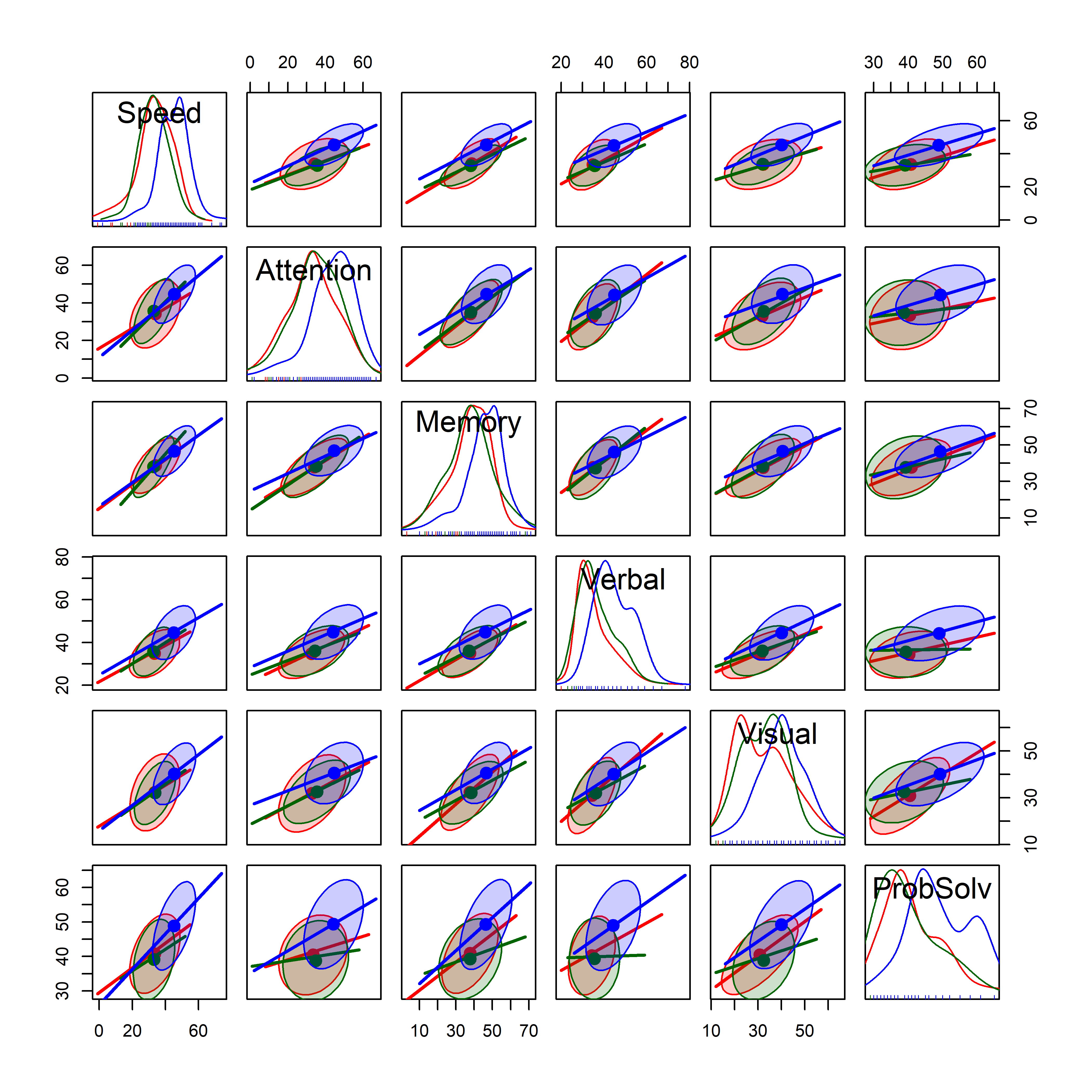
NeuroCog data. Points are suppressed here, focusing on the data ellipses and regression lines. Colors for the groups: Schizophrenic SchizoAffective Control
In Figure fig-NC-scatmat, you can see that the regression lines have similar slopes and similar data ellipses for the groups, though with a few exceptions. You can also see that the Normal group has higher means on all the variables and that the Schizophrenic and SchizoAffective don’t seem to differ very much.
Biplot
While still in exploratory mode, we can gain greater insight with our trusty multivariate juicer, the biplot (sec-biplot). A PCA of the cognitive variables shows that nearly 80% of the total variance is accounted for by two dimensions, of which the first dimension accounts for 69%.
neuro.pca <- NeuroCog |>
  select(Speed:Visual) |>
  prcomp(scale. = TRUE)
summary(neuro.pca)
# Importance of components:
#                          PC1   PC2   PC3    PC4    PC5
# Standard deviation     1.856 0.720 0.629 0.5761 0.5570
# Proportion of Variance 0.689 0.104 0.079 0.0664 0.0621
# Cumulative Proportion  0.689 0.793 0.872 0.9379 1.0000
The biplot for this analysis (Figure fig-neuro-biplot) provides a nice summary of what was seen in the scatterplot matrix (Figure fig-NC-scatmat): A large difference between the Control group and the others, which don’t differ much from each other.
ggbiplot(neuro.pca,
         obs.scale = 1, var.scale = 1,
         groups = NeuroCog$Dx,
         varname.size = 5,
         var.factor = 1.5,
         ellipse = TRUE) +
  scale_color_discrete(name = 'groups') +
  theme_minimal() +
  theme(legend.direction = 'horizontal',
        legend.position = 'top')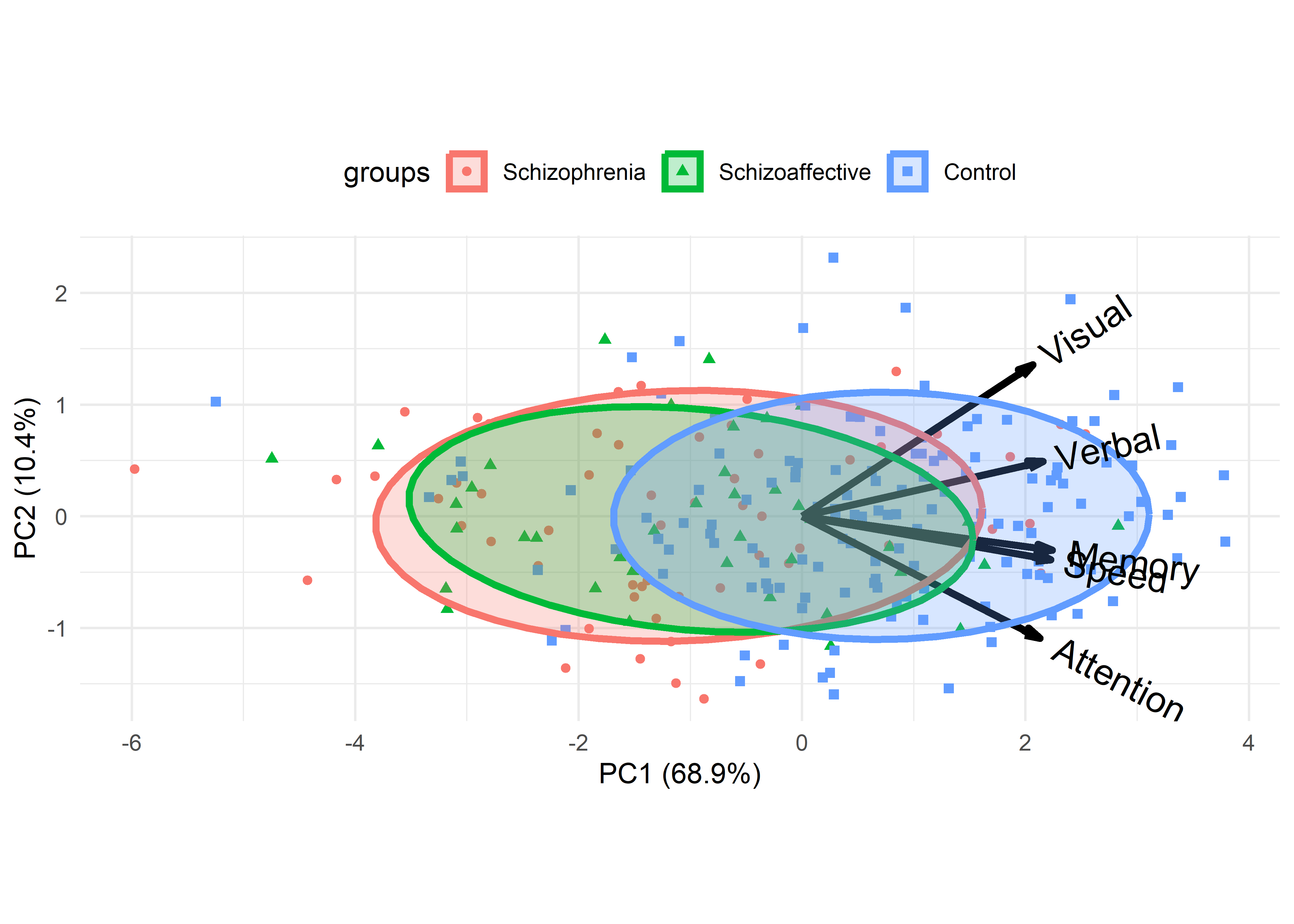
The variable vectors in Figure fig-neuro-biplot reflect the correlations of the response variables with each other and with the principal components, PC1 and PC2. All of the variables are positively correlated in this 2D view, Memory and Speed most highly so.
14.3 Fitting the MLM
We proceed to fit the one-way MANOVA model to answer the main research question of how well these variables distinguish among the groups.
NC.mlm <- lm(cbind(Speed, Attention, Memory, Verbal, Visual, ProbSolv) ~ Dx,
             data=NeuroCog)
Anova(NC.mlm)
#
# Type II MANOVA Tests: Pillai test statistic
#    Df test stat approx F num Df den Df  Pr(>F)
# Dx  2     0.299     6.89     12    470 1.6e-11 ***
# ---
# Signif. codes:  0 '***' 0.001 '**' 0.01 '*' 0.05 '.' 0.1 ' ' 1
The first research question is captured by the contrasts for the Dx factor shown above. We can test these with car::linearHypothesis(). The contrast Dx1 for control vs. the diagnosed groups is highly significant,
# control vs. patients
print(linearHypothesis(NC.mlm, "Dx1"), SSP=FALSE)
#
# Multivariate Tests:
#                  Df test stat approx F num Df den Df  Pr(>F)
# Pillai            1     0.289     15.9      6    234 2.8e-15 ***
# Wilks             1     0.711     15.9      6    234 2.8e-15 ***
# Hotelling-Lawley  1     0.407     15.9      6    234 2.8e-15 ***
# Roy               1     0.407     15.9      6    234 2.8e-15 ***
# ---
# Signif. codes:  0 '***' 0.001 '**' 0.01 '*' 0.05 '.' 0.1 ' ' 1
However, the second contrast, Dx2, comparing the schizophrenic and schizoaffective group, shows no difference in the collection of response means.
# Schizo vs SchizAff
print(linearHypothesis(NC.mlm, "Dx2"), SSP=FALSE)
#
# Multivariate Tests:
#                  Df test stat approx F num Df den Df Pr(>F)
# Pillai            1     0.006    0.249      6    234   0.96
# Wilks             1     0.994    0.249      6    234   0.96
# Hotelling-Lawley  1     0.006    0.249      6    234   0.96
# Roy               1     0.006    0.249      6    234   0.96
As a quick check on the model, a \(\chi^2\) QQ plot (Figure fig-NC-cqplot) reveals no problems with multivariate normality of residuals nor potentially harmful residuals.
cqplot(NC.mlm, id.n = 3)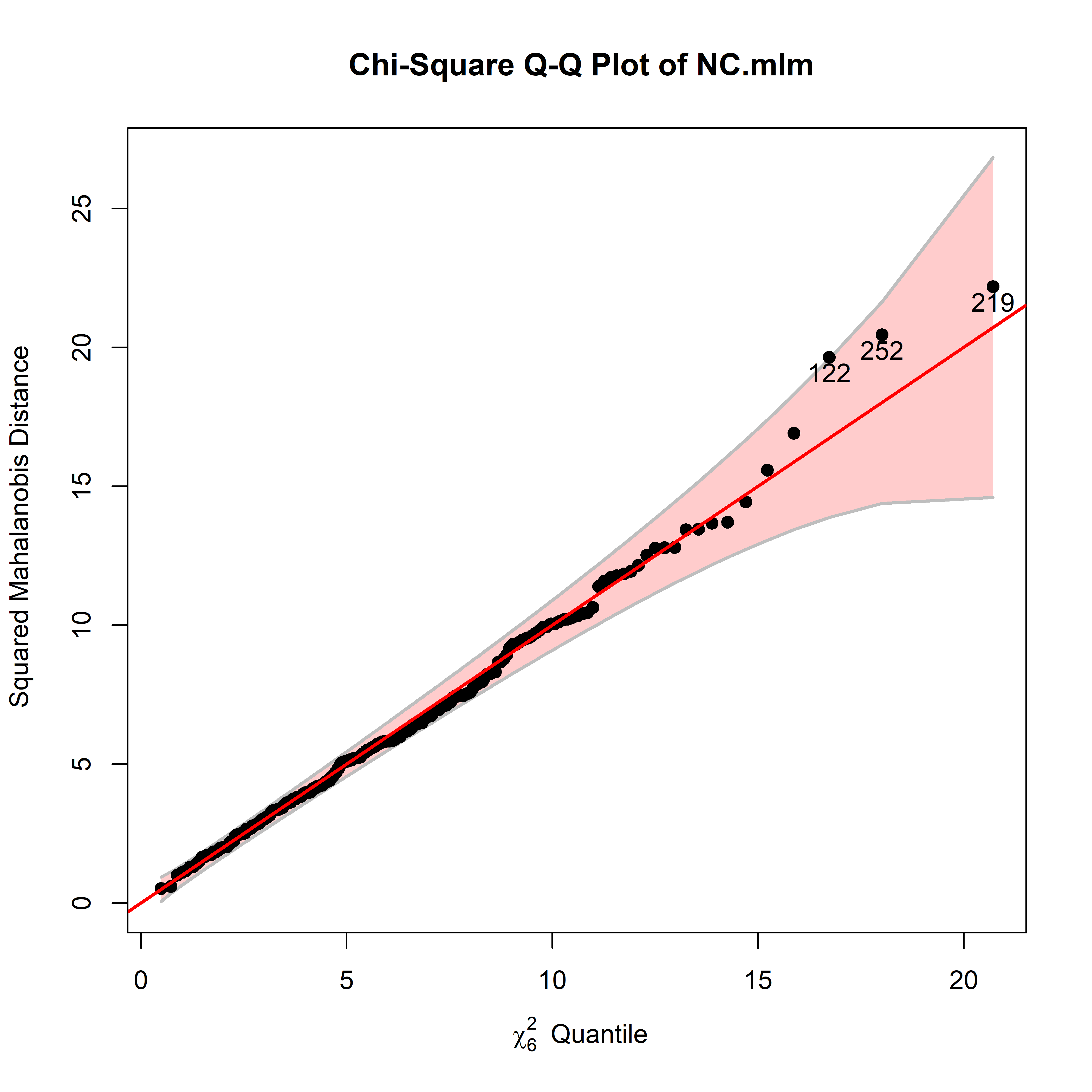
14.3.1 HE plot
So the question becomes: how to understand these results.heplot() shows the visualization of the multivariate model in the space of two response variables (the first two by default). The result (Figure fig-NC-HEplot) tells a very simple story: The control group performs higher on higher measures than the diagnosed groups, which do not differ between themselves.
(Because heplot() gets the levels of factors from the model object, in order to abbreviate the group labels in the plot, you need to update() the MLM model after the labels are reassigned.)
Then, feed the model to heplot() for a plot of the first two response variables, Speed and Attention.
heplot(NC.mlm,
       fill=TRUE, fill.alpha=0.1,
       cex.lab=1.5, cex=1.35)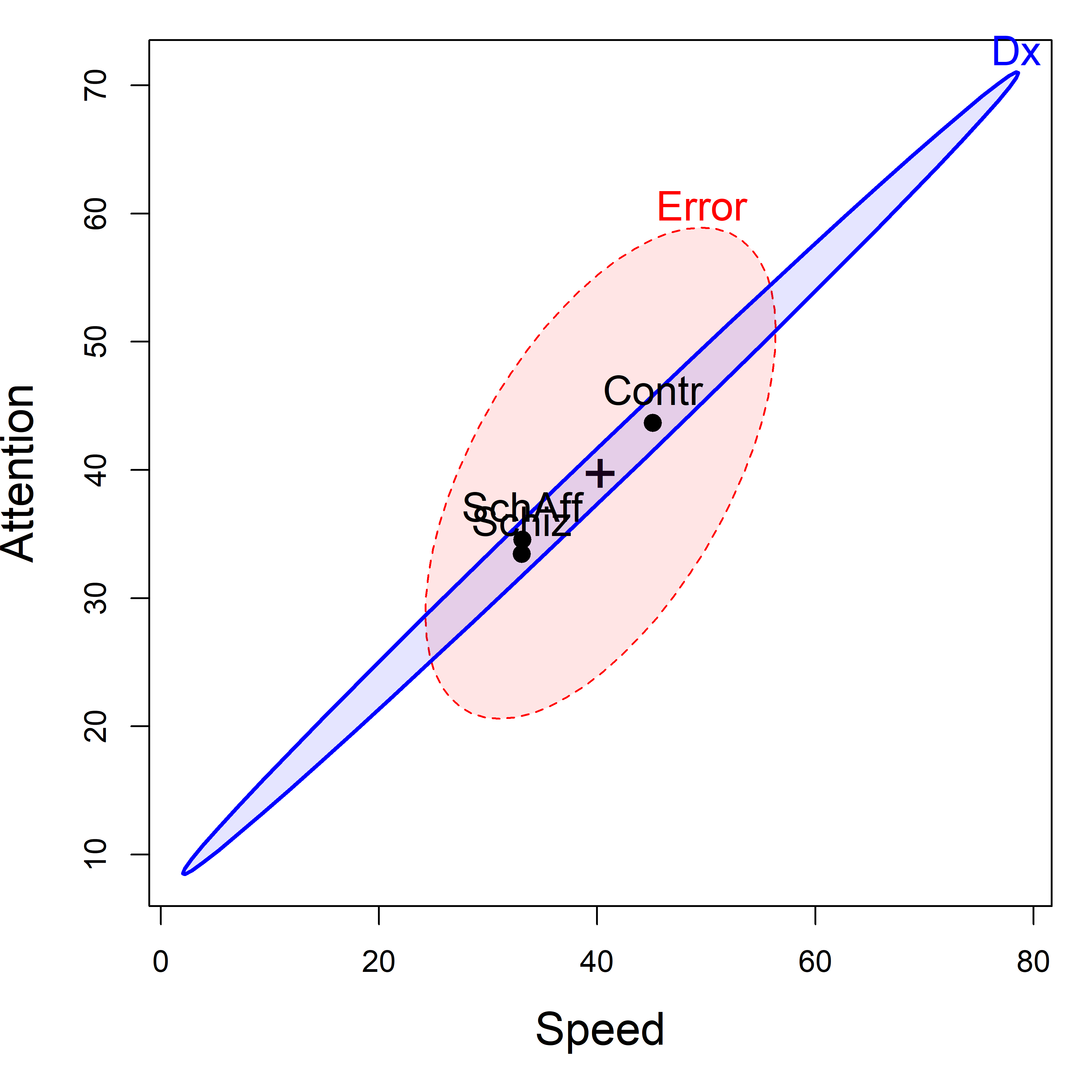
NeuroCog data. The labeled points show the means of the groups on the two variables. The blue \(\mathbf{H}\) ellipse for groups indicates the strong positive correlation of the group means.
This pattern, of the control group higher than the others, is consistent across all of the response variables, as we see from a plot of pairs(NC.mlm) in Figure fig-NC-HE-pairs.
pairs(NC.mlm,
      fill=TRUE, fill.alpha=0.1,
      var.cex=2)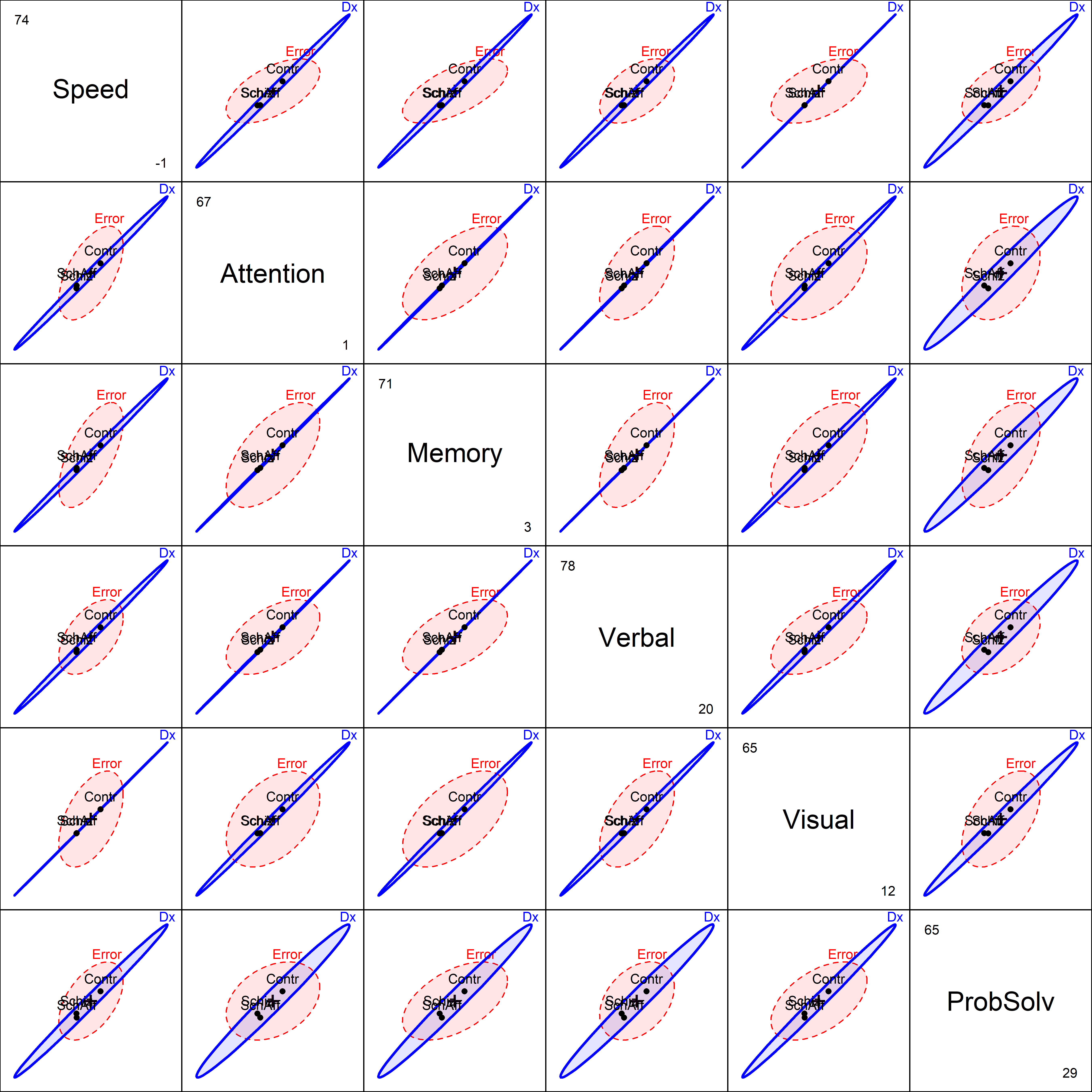
NeuroCog data. The visual evidence that these outcome measures are strongly related in distinguishing the groups is very clear.
The group means are nearly perfectly correlated in all panels. This signals that we are likely to see a very simple representation of the data in canonical space. Note that this differs from the biplot view (Figure fig-neuro-biplot) in that biplot ignores the Dx factor in the PCA, even though we represent it in the plot.
14.3.2 Canonical space
We can gain further insight, and a simplified plot showing all the response variables by projecting the MANOVA into the canonical space, which is entirely 2-dimensional (because \(\text{df}_h=2\)). However, the output from candisc() shows that 98.5% of the mean differences among groups can be accounted for in just one canonical dimension.
NC.can <- candisc(NC.mlm)
NC.can
#
# Canonical Discriminant Analysis for Dx:
#
#    CanRsq Eigenvalue Difference Percent Cumulative
# 1 0.29295    0.41433      0.408    98.5       98.5
# 2 0.00625    0.00629      0.408     1.5      100.0
#
# Test of H0: The canonical correlations in the
# current row and all that follow are zero
#
#   LR test stat approx F numDF denDF Pr(> F)
# 1        0.703     7.53    12   468   9e-13 ***
# 2        0.994     0.30     5   235    0.91
# ---
# Signif. codes:  0 '***' 0.001 '**' 0.01 '*' 0.05 '.' 0.1 ' ' 1
Figure fig-NC-candisc is the result of the plot() method for class "candisc" objects, that is, the result of calling plot(NC.can, ...). It plots the two canonical scores, \(\mathbf{Z}_{n \times 2}\) for the subjects, together with data ellipses for each of the three groups.
pos <- c(4, 1, 4, 4, 1, 3)
col <- c("red", "darkgreen", "blue")
plot(NC.can,
     ellipse=TRUE,
     rev.axes=c(TRUE,FALSE),
     pch=c(7,9,10),
     var.cex=1.2, cex.lab=1.5, var.lwd=2,  scale=4.5,
     col=col,
     var.col="black", var.pos=pos,
     prefix="Canonical dimension ")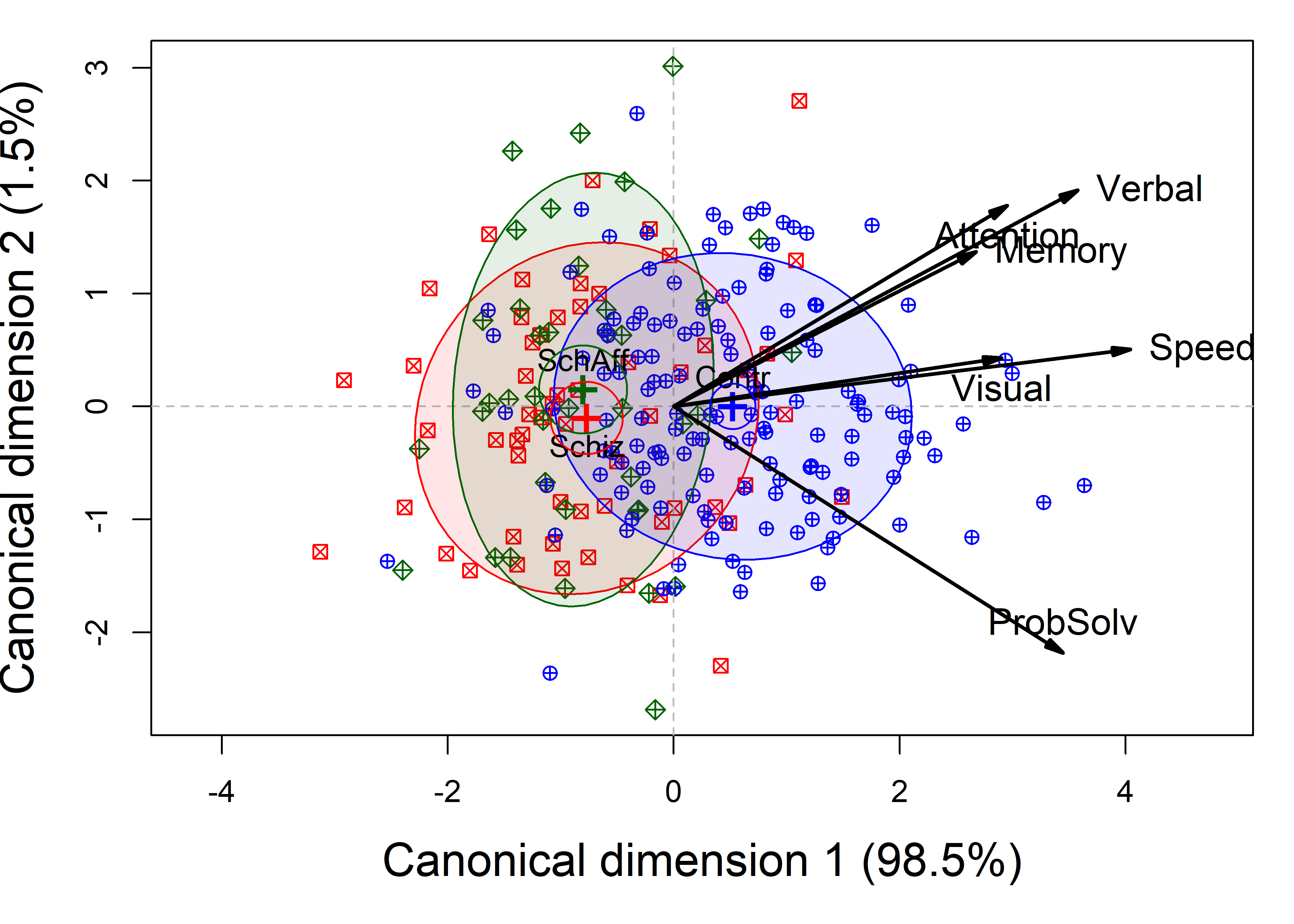
NeuroCog data MANOVA. Scores on the two canonical dimensions are plotted, together with 68% data ellipses for each group.
The interpretation of Figure fig-NC-candisc is again fairly straightforward. As noted earlier (sec-candisc), the projections of the variable vectors in this plot on the coordinate axes are proportional to the correlations of the responses with the canonical scores. From this, we see that the normal group differs from the two patient groups, having higher scores on all the neurocognitive variables, most of which are highyl correlated. The problem solving measure is slightly different, and this, compared to the cluster of memory, verbal and attention, is what distinguishes the schizophrenic group from the schizoaffectives.
The separation of the groups is essentially one-dimensional, with the control group higher on all measures. Moreover, the variables processing speed and visual memory are the purest measures of this dimension, but all variables contribute positively. The second canonical dimension accounts for only 1.5% of group mean differences and is non-significant (by a likelihood ratio test). Yet, if we were to interpret it, we would note that the schizophrenia group is slightly higher on this dimension, scoring better in problem solving and slightly worse on working memory, attention, and verbal learning tasks.
Summary
This analysis gives a very simple description of the data, in relation to the research questions posed earlier:
On the basis of these neurocognitive tests, the schizophrenic and schizoaffective groups do not differ significantly overall, but these groups differ greatly from the normal controls.
All cognitive domains distinguish the groups in the same direction, with the greatest differences shown for the variables most closely aligned with the horizontal axis in Figure fig-NC-candisc. This means that these neuro-psychological measures can be considered to tap a single dimension of differences among the three diagnostic groups.
14.4 Social cognitive measures
The social cognitive measures in the Hartman (2016) study were designed to tap various aspects of the perception and cognitive processing of emotions of others. Emotion perception was assessed using a Managing Emotions score from the MCCB. A “theory of mind” (ToM) score assessed ability to read the emotions of others from photographs of the eye region of male and female faces. Two other measures, externalizing bias (ExtBias) and personalizing bias (PersBias) were calculated from a scale measuring the degree to which individuals attribute internal, personal or situational causal attributions to positive and negative social events.
The analysis of the SocialCog data proceeds in a similar way: first we fit the MANOVA model, then test the overall differences among groups using Anova(). We find that the overall multivariate test is again significant,
data(SocialCog, package="heplots")
SC.mlm <-  lm(cbind(MgeEmotions,ToM, ExtBias, PersBias) ~ Dx,
               data=SocialCog)
Anova(SC.mlm)
#
# Type II MANOVA Tests: Pillai test statistic
#    Df test stat approx F num Df den Df  Pr(>F)
# Dx  2     0.212     3.97      8    268 0.00018 ***
# ---
# Signif. codes:  0 '***' 0.001 '**' 0.01 '*' 0.05 '.' 0.1 ' ' 1
Testing the same two contrasts using linearHypothesis() (results not shown), w e find that the overall multivariate test is again significant, but now both contrasts are significant (Dx1: \(F(4, 133)=5.21, p < 0.001\); Dx2: \(F(4, 133)=2.49, p = 0.0461\)), the test for Dx2 just barely.
# control vs. patients
print(linearHypothesis(SC.mlm, "Dx1"), SSP=FALSE)
# Schizo vs. SchizAff
print(linearHypothesis(SC.mlm, "Dx2"), SSP=FALSE)
These results are important, because, if they are reliable and make sense substantively, they imply that patients with schizophrenia and schizoaffective diagnoses can be distinguished by their performance on tasks assessing social perception and cognition. This was potentially a new finding in the literature on schizophrenia.
As we did above, it is useful to visualize the nature of these differences among groups with HE plots for the SC.mlm model. Each contrast has a corresponding \(\mathbf{H}\) ellipse, which we can show in the plot using the hypotheses argument. With a single degree of freedom, these degenerate ellipses plot as lines.
heplot(SC.mlm,
       hypotheses=list("Dx1"="Dx1", "Dx2"="Dx2"),
       fill=TRUE, fill.alpha=.1,
       cex.lab=1.5, cex=1.2)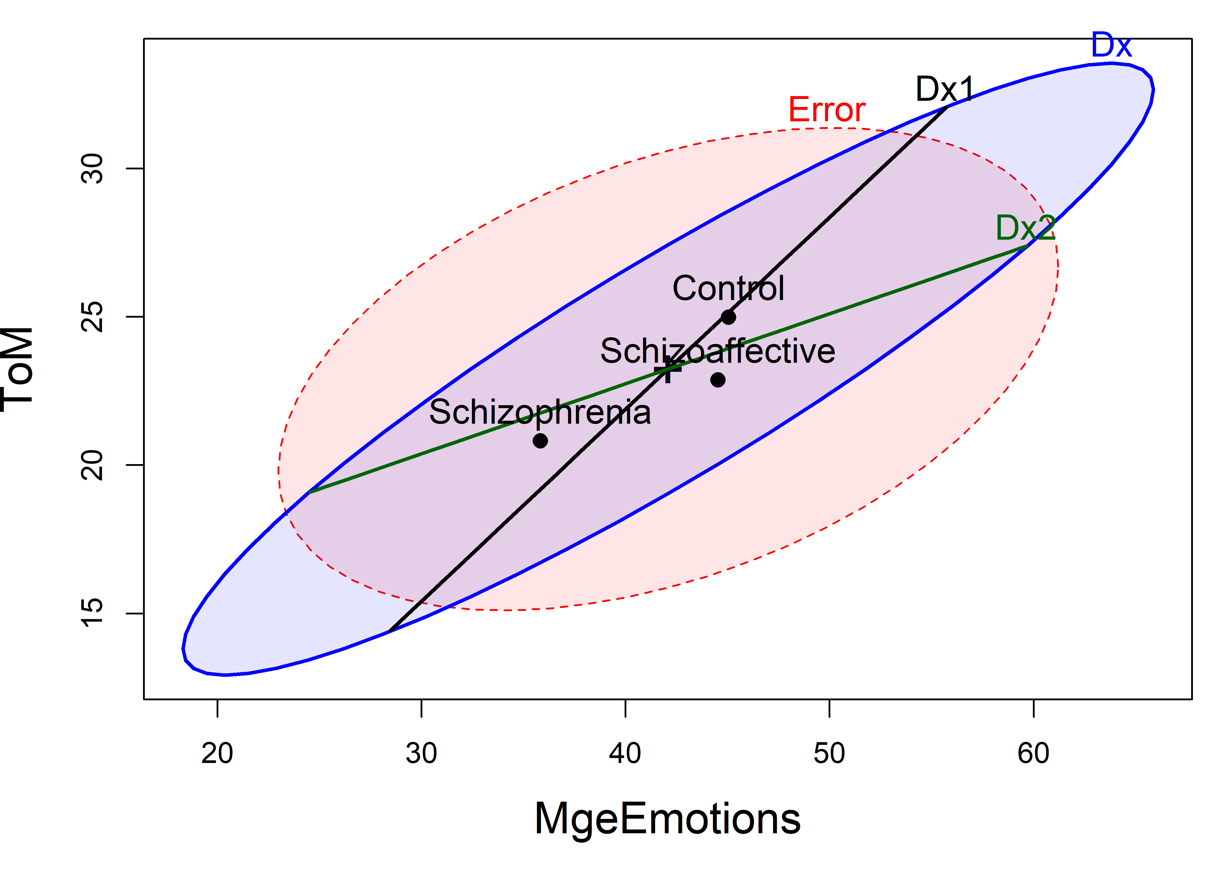
SocialCog data. The labeled points show the means of the groups on the two variables. The lines for Dx1 and Dx2 show the tests of the contrasts among groups.
It can be seen that the three group means are approximately equally spaced on the ToM measure, whereas for MgeEmotions, the control and schizoaffective groups are quite similar, and both are higher than the schizophrenic group. This ordering of the three groups was somewhat similar for the other responses, as we could see in a pairs(SC.mlm) plot.
14.4.1 Model checking
Normally, we would continue this analysis, and consider other HE and canonical discriminant plots to further interpret the results, in particular the relations of the cognitive measures to group differences, or perhaps an analysis of the relationships between the neuro- and social-cognitive measures. We don’t pursue this here for reasons of length, but this example actually has a more important lesson to demonstrate.
Before beginning the MANOVA analyses, extensive data screening was done by the client using SPSS, in which all the response and predictor variables were checked for univariate normality and multivariate normality (MVN) for both sets. This traditional approach yielded a huge amount of tabular output and no graphs, and did not indicate any major violation of assumptions.2
A simple visual test of MVN and the possible presence of multivariate outliers is related to the theory of the data ellipse: Under MVN, the squared Mahalanobis distances \(D^2_M (\mathbf{y}) = (\mathbf{y} - \bar{\mathbf{y}})' \, \mathbf{S}^{-1} \, (\mathbf{y} - \bar{\mathbf{y}})\) should follow a \(\chi^2_p\) distribution. Thus, a quantile-quantile plot of the ordered \(D^2_M\) values vs. corresponding quantiles of the \(\chi^2\) distribution should approximate a straight line (Cox, 1968; Healy, 1968). Note that this should be applied to the residuals from the model – residuals(SC.mlm) – and not to the response variables directly.
heplots::cqplot() implements this for "mlm" objects Calling this function for the model SC.mlm produces Figure fig-SC-cqplot. It is immediately apparent that there is one extreme multivariate outlier; three other points are identified, but the remaining observations are nearly within the 95% confidence envelope (using a robust MVE estimate of \(\mathbf{S}\)).
cqplot(SC.mlm, method="mve",
       id.n=4,
       main="",
       cex.lab=1.25)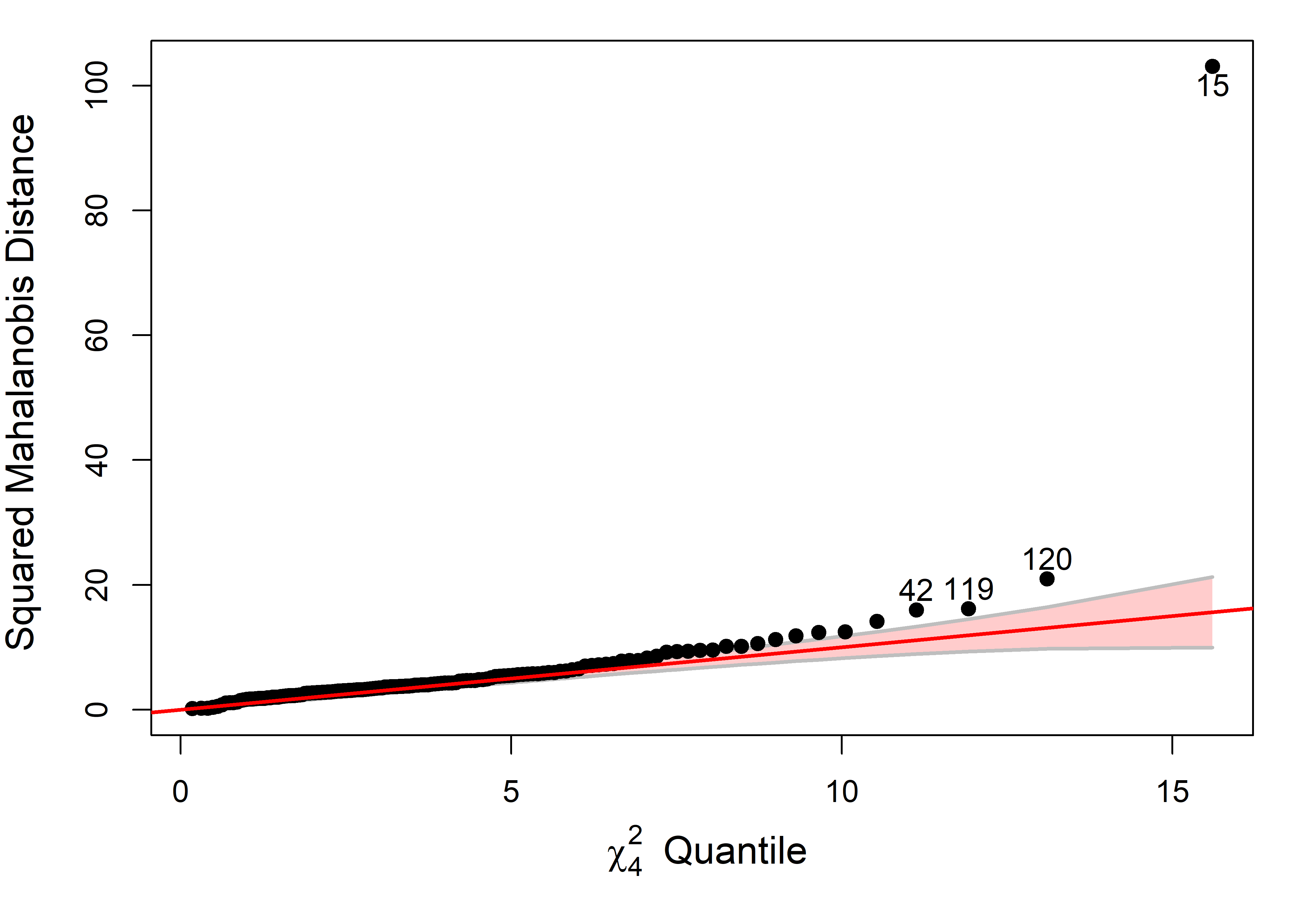
SC.mlm. The confidence band gives a point-wise 95% envelope, providing information about uncertainty. One extreme multivariate outlier is highlighted.
Further checking revealed that this was a data entry error where one case (15) in the schizophrenia group had a score of -33 recorded on the ExtBias measure, whose valid range was (-10, +10). In R, it is very easy to re-fit a model to a subset of observations (rather than modifying the dataset itself) using update(). The result of the overall Anova and the test of Dx1 were unchanged; however, the multivariate test for the most interesting contrast Dx2 comparing the schizophrenia and schizoaffective groups became non-significant at the \(\alpha=0.05\) level (\(F(4, 133)=2.18, p = 0.0742\)).
SC.mlm1 <- update(SC.mlm,
                  subset=rownames(SocialCog)!="15")

Anova(SC.mlm1)
print(linearHypothesis(SC.mlm1, "Dx1"), SSP=FALSE)
print(linearHypothesis(SC.mlm1, "Dx2"), SSP=FALSE)
14.4.2 Canonical HE plot
This outcome creates a bit of a quandry for further analysis (do univariate follow-up tests? try a robust model?) and reporting (what to claim about the Dx2 contrast?) that we don’t explore here. Rather, we proceed to attempt to interpret the MLM with the aid of canonical analysis and a canonical HE plot. The canonical analysis of the model SC.mlm1 now shows that both canonical dimensions are significant, and account for 83.9% and 16.1% of between group mean differences respectively.
SC.can1 <- candisc(SC.mlm1)
SC.can1
#
# Canonical Discriminant Analysis for Dx:
#
#   CanRsq Eigenvalue Difference Percent Cumulative
# 1 0.1645     0.1969      0.159    83.9       83.9
# 2 0.0364     0.0378      0.159    16.1      100.0
#
# Test of H0: The canonical correlations in the
# current row and all that follow are zero
#
#   LR test stat approx F numDF denDF Pr(> F)
# 1        0.805     3.78     8   264 0.00032 ***
# 2        0.964     1.68     3   133 0.17537
# ---
# Signif. codes:  0 '***' 0.001 '**' 0.01 '*' 0.05 '.' 0.1 ' ' 1
op <- par(mar=c(5,4,1,1)+.1)
heplot(SC.can1,
fill=TRUE, fill.alpha=.1,
hypotheses=list("Dx1"="Dx1", "Dx2"="Dx2"),
lwd = c(1, 2, 3, 3),
col=c("red", "blue", "darkgreen", "darkgreen"),
var.lwd=2,
var.col="black",
label.pos=c(3,1),
var.cex=1.2,
cex=1.25, cex.lab=1.2,
scale=2.8,
prefix="Canonical dimension ")
par(op)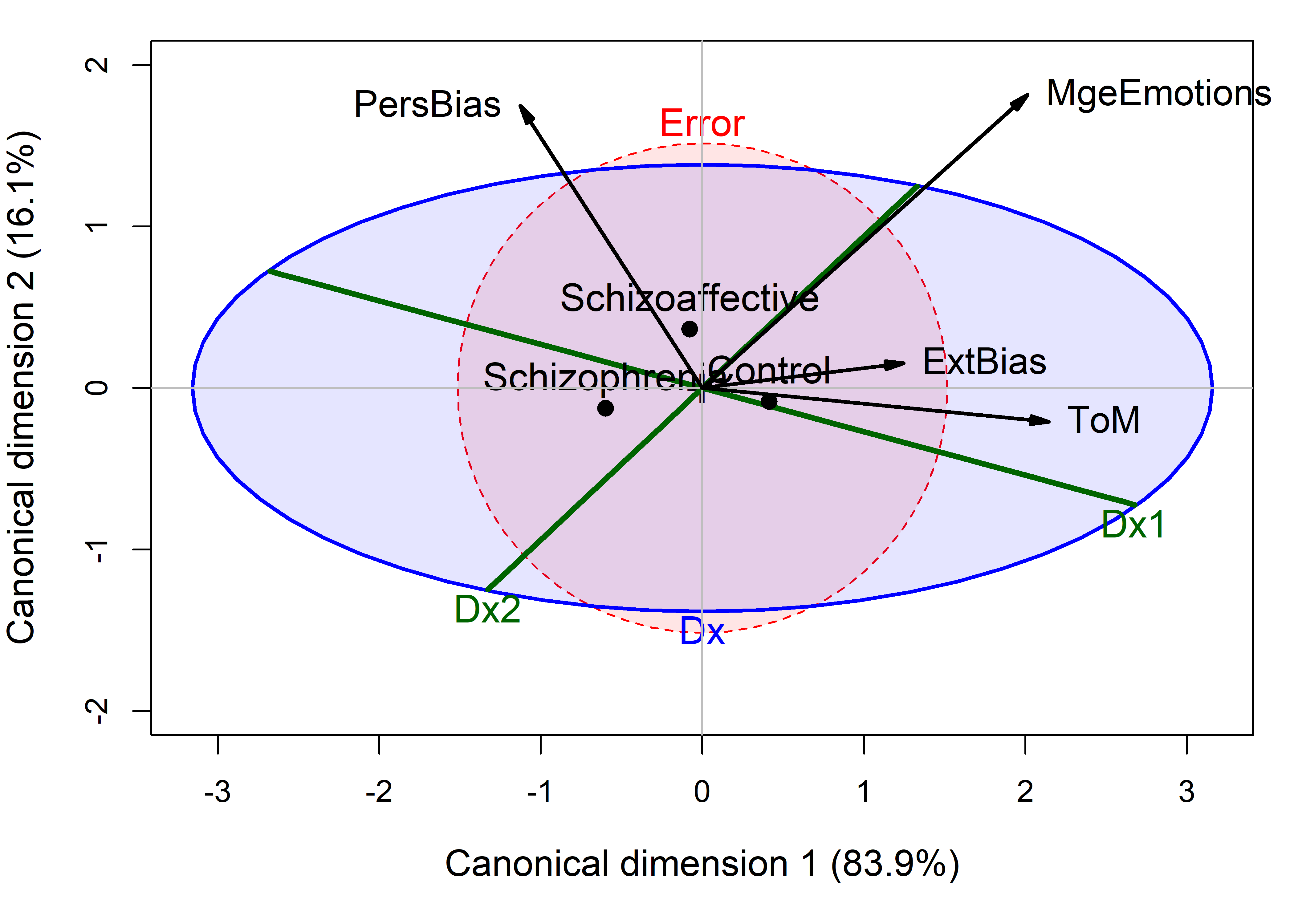
SocialCog MANOVA. The variable vectors show the correlations of the responses with the canonical variables. The embedded green lines show the projections of the H ellipses for the contrasts Dx1 and Dx2 in canonical space.
The HE plot version of this canonical plot is shown in Figure fig-SC1-hecan. Because the heplot() method for a "candisc" object refits the original model to the \(\mathbf{Z}\) canonical scores, it is easy to also project other linear hypotheses into this space. Note that in this view, both the Dx1 and Dx2 contrasts project outside \(\mathbf{E}\) ellipse.3.
This canonical HE plot has a very simple description:
- Dimension 1 orders the groups from control to schizoaffective to schizophrenia, while dimension 2 separates the schizoaffective group from the others;
- Externalizing bias and theory of mind contributes most to the first dimension, while personal bias and managing emotions are more aligned with the second; and,
- The relations of the two contrasts to group differences and to the response variables can be easily read from this plot.
More worked out examples are contained in the heplots vignettes
vignette("HE_manova", package="heplots")andvignette("HE_mmra", package="heplots")↩︎Actually, multivariate normality of the predictors in \(\mathbf{X}\) is not required in the MLM. This assumption applies only to the conditional values \(\mathbf{Y} \;|\; \mathbf{X}\), i.e., that the errors \(\boldsymbol{\epsilon}_{i}' \sim \mathcal{N}_{p}(\mathbf{0},\boldsymbol{\Sigma})\) with constant covariance matrix. Moreover, the widely used MVN test statistics, such as Mardia’s (1970) test based on multivariate skewness and kurtosis are known to be quite sensitive to mild departures in kurtosis (Mardia, 1974) which do not threaten the validity of the multivariate tests.↩︎
The direct application of significance tests to canonical scores probably requires some adjustment because these are computed to have the optimal between-group discrimination.↩︎